Run Shiny app on a Ubuntu server on the Amazon Cloud

This guide is more for self reference than anything else. 
Since I struggled for two days trying to find all the correct setting to complete this task, gathering information from several websites, I decided to write a little guide on this blog so that if I want to do it again in the future and I do not remember anything (this happens a lot!!) at least I have something to resuscitate my memory.

I found most of the information and code I used from these websites:
http://tylerhunt.co/2014/03/amazon-web-services-rstudio/
http://www.howtogeek.com/howto/41560/how-to-get-ssh-command-line-access-to-windows-7-using-cygwin/
http://www.rstudio.com/products/shiny/download-server/


Preface
First I would like to point out that this guide assumes you (I am talking to myself of the future) remember how to open an instance in the Amazon Cloud. It is not that difficult, you go to this page:
http://aws.amazon.com/ec2/

you log in (if you remember the credentials) and you should see the "Amazon Web Services" page, here you can select EC2 and launch an instance. Remember to select the correct server from the menu on the top right corner since the last time you run all the instances from Oregon, and you live in freaking Switzerland!!


Guide
NOTE
Instead of installing cygwin and cover step 1 and 2 we can just first cover step 4 and connect to the ubuntu server using WinSCP, then start putty from WinSCP and it will be already connected.


1) Install Cygwin
This software is needed to communicate with the Ubuntu server.
It is important to follow the instructions on this page (http://www.howtogeek.com/howto/41560/how-to-get-ssh-command-line-access-to-windows-7-using-cygwin/) to install the software correctly.
In particular during the installation process a "select packages" windows appears where we need to select openssh and click on "skip", until there is a cross on the column bin.

When Cygwin is installed we need to click with the right button on the icon and select "run as administrator", then open it.
Now we can run the following line to install ssh:

ssh-host-config

During the process several questions will be asked, the following answers apply:
- Should privilege separation be used? YES
- New local account sshd? YES
- Run ssh as a service? YES
- Enter a value for daemon:  ntsec
- Do you want to use a different name? NO
- Create a new privilege account user? YES  -> then insert a password


After the installation we need to insert the following line to start the sshd service:

net start sshd

Then this line to configure the service:

ssh-user-config

Again it will ask a series of questions. There is a difference between the new version and what is written on the website.
Now it asks only about an SSH2 RSA identity file to be created, the answer is YES.
Then it asks other two questions regarding DSA files and another thing, the answers here are two NO.



2) Connect to the Amazon Server
Open Cygwin.
Go to the folder where the .pem file is saved, using the following line:

cd D:/<folder>/<folder>



NOTE:
Cygwin does not like folder names with spaces!


Now we need to be sure that the .pem key will not be publicly available using the following line

chmod 400 <NAME>.pem

and then we can connect to the ubuntu server using the following line:

ssh -i <NAME>.pem ubuntu@<PUBLIC IP>

These information are provided in Amazon if we click on "Connect" once the instance has properly been launched.
Once we are in we can installing R and Shiny.


3) Install R and Shiny
The first thing to do is set up the root user with the following line:

sudo passwd root

The system will ask to input a password.
Then we can log in using the following line:

su

Now we are logged in as root users.

Now we need to update everything with the following:

apt-get update

At this point we can install R with the following line:

apt-get install r-base


NOTE:
It may be that during the installation process an older version of R is installed and this may create problems with some packages.
To solve this problem we need to modify the file sources.list located in /etc/apt/sources.list
We can do this by using WinSCP, but first we need to be sure that we have access to the folder.
We should run the following two lines:

cd /etc/

chmod 777 apt

This gives us access to modify the files in the folder apt via WinSCP (see point 4).
This line of code gives indiscriminate access to the folder, so it is not super secure.

Now we can connect and add the following line at the end:

deb http://cran.stat.ucla.edu/bin/linux/ubuntu trusty/

Then we need to first remove the old version of R using:

apt-get remove r-base

or

apt-get remove r-base-dev

Then we need to run once again both the update and the installation calls.



We can check the amount of disk space left on the server using the following command:

df -h


Then we can start R just by typing R in the console.
At this point we need to install all the packages we would need to run shiny using standard R code:

install.packages("raster")


Now we can exit from R with q() and install shiny suing the following line in ubuntu:

sudo su - \
-c "R -e \"install.packages('shiny', repos='http://cran.rstudio.com/')\""

Now we need to install gdebi with the following lines (check here for any update:http://www.rstudio.com/products/shiny/download-server/):

apt-get install gdebi-core
wget http://download3.rstudio.org/ubuntu-12.04/x86_64/shiny-server-1.3.0.403-amd64.deb
gdebi shiny-server-1.3.0.403-amd64.deb



4) Transfer file between windows and Ubuntu
We can use WinSCP (http://winscp.net/eng/index.php) for this task.

First of all we need to import the .pem file that is need for the authentication.
From the "New Site" window we can go to "advanced", then click on "SSH -> Authentication".
From the "Private key file" we can browse and open the .pem file. We need to transform it into a ppk file but we can do that using the default settings.
We can just click on "Save private key" to save the ppk file and then import it again on the same field, and click OK.

Now the Host name is the name of the instance, for example:
ec2-xx-xx-xxx-xxx.eu-west-1.compute.amazonaws.com

The user name is ubuntu and the password is left blank. The protocol is SFTP and the port is 22.

The shiny server is located in the folder /srv/shiny-server

We need to give WinSCP access to this folder using again the command

cd srv
chmod 777 shiny-server





5) Transfer shiny app files on the server
In WinSCP open the folder /srv/shiny-server and create a new folder with the name of your shiny app.
Then transfer the files from your PC to the folder.
Remember to change the address of the files or working directory in the R script with the new links.


6) Allow the port 3838 to access the web
To do this we need to change the rule in the "security groups" menu.
This menu is visible in the main window where all your instances are shown. However, do not access the menu from the panel of the left, that area may be a bit confusing.
Instead select the instance in which you need to add the rule, look at the window at the bottom of the page (the one that shows the name of the instance) and click on the name in light blue near "security group".
This will open the security group menu specific for the instance you selected.
Here we need to add a rule by clicking on "add rule", select custom TCP, write the port number 3838 in the correct area and the select "anywhere" in the IP section.

Now if you go to the following page you should see the app:
<PUBLIC IP>:3838/<FOLDER>

It is sometimes necessary to open port 22 as well, using the same procedure to keep connecting to the server with cygwin or putty.


7) Stop, start and restart Shiny server

sudo start shiny-server

sudo stop shiny-server

sudo restart shiny-server


8) Installing rgdal
This package require some tweaks before its installations. On this site I found what I needed: http://askubuntu.com/questions/206593/how-to-install-rgdal-on-ubuntu-12-10

Basically from the Ubuntu console just run these three lines of code:
sudo apt-get install aptitude
sudo aptitude install libgdal-dev
sudo aptitude install libproj-dev

Then go back to R and install rgdal normally (with install.packages)



9) Installing rCharts
Before installing rCharts we need to run the line above to install rgdal (I also run the first two lines suggested in the comments, but I do not know if it helped). I also run the following lines from here: http://stackoverflow.com/questions/16363144/install-rcharts-package-on-r-2-15-2

sudo apt-get install libcurl4-openssl-dev
sudo apt-get install openjdk-6-jdk
export LD_LIBRARY_PATH=/usr/lib/jvm/java-6-openjdk-amd64/jre/lib/amd64/server
R CMD javareconf 

but I do not know if they helped or not. 

If we not do that "devtools" will not install and therefore we will not be able to install rCharts from github:

require(devtools)
install_github('rCharts', 'ramnathv')

To run rCharts from the ubuntu server we need to make sure that the links to the javascript library are not referring to


NOTE:
You may need to add packages in R after the installation. For doing that you always need to remember to access ubuntu as root user, so first thing to do is write the code:

su

and insert the password. Now you can start R and install the packages. Otherwise the lib folder where the packages are installed would not be accessible.




#UPDATE from Mike Rutter
To make the install easier, add the following PPAs:

sudo apt-add-repository ppa:marutter/rrutter
sudo apt-add-repository ppa:marutter/c2d4u

The first is the same as the CRAN repository, but you don't need to edit "sources.list". The second has over 2,500 R packages ready to install. For example:

sudo apt-get install r-cran-raster r-cran-rgdal r-cran-shiny

will install the R packages mentioned in the the post. No need to install the "dev" packages either, as that will be taken care of by apt. And the will be updated via the regular Ubuntu update process.

NOTE
Without updating the file in /etc/apt we can just run the first two lines suggested by Mike, then remove r-base and re-install it to have the updated version.

Extract values from numerous rasters in less time

These days I was working with a Shiny app for which the computation time is a big problem.
Basically this app takes some coordinates, extract values from 1036 rasters for these coordinates and make some computations. 
As far as I can (and please correct me if I'm wrong!) tell there are two ways of doing this task:
1) load all the 1036 rasters and extract the values from each of them in a loop
2) create a stack raster and extract the values only one time

In the first approach it helps if I have all my rasters in one single folder, since in that case I can run the following code:

f <- list.files(getwd()) 
ras <- lapply(f,raster) 
ext <- lapply(ras,extract,MapUTM) 
ext2 <- unlist(ext)
t1 <- Sys.time()

The first line creates a list of all the raster file in the working directory, then with the second line I can read them in R using the package raster.
The third line extracts from each raster the values that corresponds to the coordinates of the SpatialPoints object named MapUTM. The object ext is a list, therefore I have to change it into a numeric vector for the computations I will do later in the script.
This entire operation takes 1.835767 mins.

Since this takes too much time I thought of using a stack raster. I can just run the following line to create
a RasterStack object with 1036 layers. This is almost instantaneous.

STACK <- stack(ras)

The object looks like this:

> STACK
class       : RasterStack 
dimensions  : 1217, 658, 800786, 1036  (nrow, ncol, ncell, nlayers)
resolution  : 1000, 1000  (x, y)
extent      : 165036.8, 823036.8, 5531644, 6748644  (xmin, xmax, ymin, ymax)
coord. ref. : NA 
names       :      Dir_10,      Dir_11,      Dir_12,      Dir_13,      Dir_14,      Dir_15,      Dir_16,      Dir_17,      Dir_18,      Dir_19,      Dir_20,      Dir_21,      Dir_22,      Dir_23,      Dir_24, ... 
min values  :   59.032657,  141.913933,   84.781970,  147.634633,   39.723591,  154.615133,   45.868360,  197.306633,   85.839959,  272.336367,   93.234409,  339.732100,   79.106781,  566.522933,  175.075968, ... 
max values  :  685.689288, 2579.985700,  840.835621, 3575.341167, 1164.557067, 5466.193933, 2213.728126, 5764.541400, 2447.792437, 4485.639133, 1446.003349, 5308.407167, 1650.665136, 5910.945967, 2038.332471, ... 

At this point I can extract the coordinates from all the rasters in one go, with the following line:

ext <- extract(STACK,MapUTM)

This has the advantage of creating a numeric vector, but unfortunately this operation is only slightly faster than the previous one, with a total time of 1.57565 mins

At this point, from a suggestion of a colleague Kirill Müller (http://www.ivt.ethz.ch/people/muelleki), I tested ways of translating the RasterStack into a huge matrix and then query it to extract values.
I encountered two problems with this approach, first is the amount of RAM needed to create the matrix and second is identify the exact row to extract from it.
In the package raster I can transform a Raster object into a matrix simply by calling the function as.matrix. However my RasterStack object has 800786 cells and 1036 layers, meaning that I would need to create a 800786x1036 matrix and I do have enough RAM for that.
I solved this problem using the package ff. I can create a matrix object in R that is associated with a physical object on disk. This approach allowed me to use a minimum amount of RAM and achieve the same results. This is the code I used:

mat <- ff(vmode="double",dim=c(ncell(STACK),nlayers(STACK)),filename=paste0(getwd(),"/stack.ffdata"))
 
for(i in 1:nlayers(STACK)){
mat[,i] <- STACK[[i]][]
}
save(mat,file=paste0(getwd(),"/data.RData"))

With the first line I create an empty matrix with the characteristics above (800786 rows and 1036 columns) and place it on disk.
Then in the loop I fill the matrix row by row. There is probably a better way of doing it but this does the job and that is all I actually care about. finally I save the ff object into an RData object on disk, simply because I had difficulties loading the ff object from disk.
This process takes 5 minutes to complete, but it is something you need to do just once and then you can load the matrix from disk and do the rest.

At this point I had the problem of identifying the correct cell from which to extract all the values. I solved it by creating a new raster and fill it with integers from 1 to the maximum number of cells. I did this using the following two lines:

ID_Raster <- raster(STACK[[1]])
ID_Raster[] <- 1:ncell(STACK[[1]])

Now I can use the extract function on this raster to identify the correct cell and the extract the corresponding values from the ff matrix, with the following lines:

ext_ID <- extract(ID_Raster,MapUTM)
ext2 <- mat[as.numeric(ext_ID),]

If I do the extract this way I complete the process in 2.671 secs, which is of great importance for the Shiny interface.


R code snippets created by Pretty R at inside-R.org

Downloading and Visualizing Seismic Events from USGS

The unlucky events that took place in Nepal have flooded the web with visualization of the earthquakes from USGS. They normally visualize earthquakes with a colour scale that depends on the age of the event and a marker size that depends on magnitude. I remembered that some time ago I tested ways for downloading and visualizing data from USG in the same way in R. So I decided to take those tests back, clean them up and publish them. I hope this will not offend anyone, I do not want to disrespect the tragedy, just share my work.

The USGS provides access to csv files for seismic events recording in several time frames: past hour, past day, past week, and in the past 30 days. For each of these, several choices of significance are provided, user can download all the events in the time frame or limit their request to events with magnitude higher than: 1.0, 2.5, 4.5 and significant events. The data are provided in csv files with standard names so that they are always accessible and updated every 15 minutes with new data.
USGS provides the csv files in links with standard names. For example in this case we are downloading all the data in the last month, so the csv file’s name is: all_month.csv. If we wanted to download only the earthquakes in the last day and with a magnitude above 4.5, we would have used the file name: 4.5_day.csv. The links to all the csv provided by USGS are available here: http://earthquake.usgs.gov/earthquakes/feed/v1.0/csv.php

For this experiment we need the following packages: sp, plotrix, and raster
In R we can easily import the data by simply calling the read.table function and reading the csv file from the server:

URL <- "http://earthquake.usgs.gov/earthquakes/feed/v1.0/summary/all_month.csv"
Earthquake_30Days <- read.table(URL, sep = ",", header = T)

This will download all the seismic events in the past 30 days.
Now we can transform the data, which are stored in a data.frame, into a spatial object using the following two lines:

coordinates(Earthquake_30Days)=~longitude+latitude
projection(Earthquake_30Days)=CRS("+init=epsg:4326")

The first line transforms the object Earthquake_30Days into a SpatialPointsDataFrame. The second gives it its proper projection, which is a geographical projection like Google Maps.
At this point I want to download the borders of all the countries in the world so that I can plot the seismic events with some geographical references:

download.file("http://thematicmapping.org/downloads/TM_WORLD_BORDERS_SIMPL-0.3.zip",destfile="TM_WORLD_BORDERS_SIMPL-0.3.zip")
unzip("TM_WORLD_BORDERS_SIMPL-0.3.zip",exdir=getwd())
polygons <- shapefile("TM_WORLD_BORDERS_SIMPL-0.3.shp")

These three lines can download the border shapefile from the web, unzip it into the working directory and load it.
In this example I will visualize the earthquakes using the same technique used by the USGS, with a colour that varies with the age of the event and a size that depends on magnitude. So the first thing to do is take care of the time. If we check the format of the time variable in the USGS file we see that it is a bit uncommon:

Earthquake_30Days$time[1]
[1] 2015-04-28T12:20:43.410Z

For this reason I created a function to transform this format into something we can use:

conv.time <- function(vector){
split1 <- strsplit(paste(vector),"T")
split2 <- strsplit(split1[[1]][2],"Z")
fin <- paste0(split1[[1]][1],split2[[1]][1])
paste(as.POSIXlt(fin,formate="%Y-%m-%d%H:%M:%OS3"))
}

If I apply this function to the previous example I obtain the following:

conv.time(Earthquake_30Days$time[1])
[1] "2015-04-28 12:20:43"

Now I can create a new variable in the object with this time-stamp:

DT <- sapply(Earthquake_30Days$time,FUN=conv.time)
Earthquake_30Days$DateTime <- as.POSIXlt(DT)

Now we can start the tricky part. For plotting the events with a custom colour scale and a custom size scale, we first need to create them. Moreover, we also need to create the thresholds needed for the legend.
For the colour scale we can do all that using the following lines:

days.from.today <- round(c(Sys.time()-Earthquake_30Days$DateTime)/60,0)
colour.scale <- color.scale(days.from.today,color.spec="rgb",extremes=c("red","blue"),alpha=0.5)
colors.DF <- data.frame(days.from.today,color.scale(days.from.today,color.spec="rgb",extremes=c("red","blue")))
colors.DF <- colors.DF[with(colors.DF, order(colors.DF[,1])), ]
colors.DF$ID <- 1:nrow(colors.DF)
breaks <- seq(1,nrow(colors.DF),length.out=10)

In the first line I calculate the age of the event as the difference between the system time and the event time-stamp. In the second line I create the colour scale with the function in plotrix, from red to blue and with a certain transparency.
Then I need to create the thresholds for the legend. I first create a data.frame with age and colours, then I order it by age and insert an ID column. At this point I can create the thresholds by simply using the seq function.
I do the same thing with the size thresholds:

size.DF <- data.frame(Earthquake_30Days$mag,Earthquake_30Days$mag/5)
size.DF <- size.DF[with(size.DF, order(size.DF[,1])), ]
size.DF$ID <- 1:nrow(size.DF)
breaks.size <- seq(0,max(Earthquake_30Days$mag/5),length.out=5)

Then I can plot the whole thing:

tiff(filename="Earthquake_Map.tif",width=7000,height=4000, res=300)

#Plot
plot(polygons)
plot(Earthquake_30Days, col= colour.scale, cex=Earthquake_30Days$mag/5, pch=16, add=T)

#Title and Legend
title("Earthquakes in the last 30 days",cex.main=3)
legend.pos <- list(x=-28.52392,y=-20.59119)
rect(xleft=legend.pos$x-5, ybottom=legend.pos$y-30, xright=legend.pos$x+30, ytop=legend.pos$y+10, col="white", border=NA)
legendg(legend.pos,legend=c(round(colors.DF[colors.DF$ID %in% round(breaks,0),1],2)),fill=paste(colors.DF[colors.DF$ID %in% round(breaks,0),2]),bty="n",bg=c("white"),y.intersp=0.75,title="Age",cex=0.8) 
text(x=legend.pos$x+5,y=legend.pos$y+5,"Legend:")
legend(x=legend.pos$x+15,y=legend.pos$y,legend=breaks.size[2:5]*5,pch=points(rep(legend.pos$x+15,4),c(legend.pos$y-6,legend.pos$y-9,legend.pos$y-12,legend.pos$y-15),pch=16,cex=breaks.size[2:5]),cex=0.8,bty="n",bg=c("white"),y.intersp=1.1,title="Magnitude") 

dev.off()

I divided the magnitude by 5, so that the bubbles are not too big. The position of the legends is something that depends of the image, if you decrease the area plotted on the map their location will change and you can use geographical coordinates to change it.
The result is the following image:

Download the image here: Earthquake_Map.jpg

The full script is available here: Script

Accessing, cleaning and plotting NOAA Temperature Data

In my previous post I said that my students are using data from NOAA for their research.
NOAA in fact provides daily averages of several environmental parameters for thousands of weather stations scattered across the globe, completely free.
In details, NOAA provides the following data:

• Mean temperature for the day in degrees Fahrenheit to tenths
• Mean dew point for the day in degrees Fahrenheit to tenths
• Mean sea level pressure for the day in millibars to tenths
• Mean station pressure for the day in millibars to tenths
• Mean visibility for the day in miles to tenths
• Mean wind speed for the day in knots to tenths
• Maximum sustained wind speed reported for the day in knots to tenths
• Maximum wind gust reported for the day in knots to tenths
• Maximum temperature reported during the day in Fahrenheit to tenths
• Minimum temperature reported during the day in Fahrenheit to tenths
• Total precipitation (rain and/or melted snow) reported during the day in inches and hundredths
• Snow depth in inches to tenths

A description of the dataset can be found here: GSOD_DESC.txt
All these data are available from 1929 to 2014.

The problem with these data is that they require some processing before they can be used for any sort of computation.
For example, the stations ID and coordinates are available in a text file external to the data file, so each data file needs to be cross referenced to this text file to extract the coordinates of the weather station.
Moreover, the data files are supplied as either one single .tar file or as a series of .gz files, that if extract give a series of .op textual files, which can then be opened in R.
All these steps would require some sort of processing before they can be used in R. For example one could download the data file and extract them with 7zip.

In this blog post I would provide a way of downloading the NOAA data, cleaning them (meaning define outliers and extract the coordinates for each location), and then plot them to observe their location and spatial pattern.

The first thing we need to do is loading the necessary packages:

library(raster)
library(XML)
library(plotrix)

Then I can define my working directory:

setwd("C:/")

At this point I can download and read the coordinates file from this address: isd-history.txt

The only way of reading it is by using the function read.fwt, which is used to read "fixed width tables" in R.
Typical entries of this table are provided as examples below:

024160 99999 NO DATA NO DATA
024284 99999 MORA SW +60.958 +014.511 +0193.2 20050116 20140330
024530 99999 GAVLE/SANDVIKEN AIR FORCE BAS SW +60.717 +017.167 +0016.0 20050101 20140403

Here the columns are named as follow:

• USAF = Air Force station ID. May contain a letter in the first position
• WBAN = NCDC WBAN number
• CTRY = FIPS country ID
• ST = State for US stations
• LAT = Latitude in thousandths of decimal degrees
• LON = Longitude in thousandths of decimal degrees
• ELEV = Elevation in meters
• BEGIN = Beginning Period Of Record (YYYYMMDD)
• END = Ending Period Of Record (YYYYMMDD)

As you can see, the length of each line is identical but its content varies substantially from one line to the other. Therefore there is no way of reading this file with the read.table function.
However, in read.fwt we can define the length of each column in the dataset so that we can create a data.frame out of it.
I used the following widths:

• 6 - USAF
• 1 - White space
• 5 - WBAN
• 1 - White space
• 38 - CTRY and ST
• 7 - LAT
• 1 - White space
• 7 - LON
• 9 - White space, plus Elevation, plus another White space
• 8 - BEGIN
• 1 - White space
• 8 - END

After this step I created a data.frame with just USAF, WBAN, LAT and LON.
The two lines of code for achieving all this are presented below:

coords.fwt <- read.fwf("ftp://ftp.ncdc.noaa.gov/pub/data/gsod/isd-history.txt",widths=c(6,1,5,1,38,7,1,8,9,8,1,8),sep=";",skip=21,fill=T)<br />
coords <- data.frame(ID=paste(as.factor(coords.fwt[,1])),WBAN=paste(as.factor(coords.fwt[,3])),Lat=as.numeric(paste(coords.fwt$V6)),Lon=as.numeric(paste(coords.fwt$V8)))

As you can see, I can work directly using the data link, there is actually no need to have this file local.

After this step I can download the data files for a particular year and extract them. I can use the function download.file from XML to download the .tar file, then the function untar to extract its contents.
The code for doing so is the following:

#Download Measurements
year = 2013
download.file(paste("ftp://ftp.ncdc.noaa.gov/pub/data/gsod/",year,"/gsod_",year,".tar",sep=""),destfile=paste(getwd(),"/Data/","gsod_2013.tar",sep=""),method="auto",mode="wb")

#Extract Measurements
dir.create(paste(getwd(),"/Data/Files",sep=""))
untar(paste(getwd(),"/Data/","gsod_2013.tar",sep=""),exdir=paste(getwd(),"/Data/Files",sep=""))

I created a variable year so that I can change the year I want to investigate and the script will work in the same way.
I also included a call to dir.create to create a new folder to store the 12'511 data files included in the .tar file.
At this point I created a loop to iterate through the file names.

#Create Data Frame
files <- list.files(paste(getwd(),"/Data/Files/",sep=""))

classes <- c(rep("factor",3),rep("numeric",14),rep("factor",3),rep("numeric",2))

t0 <- Sys.time()
station <- data.frame(Lat=numeric(),Lon=numeric(),TempC=numeric())
for(i in 1:length(files)){

data <- read.table(gzfile(paste(getwd(),"/Data/Files/",files[i],sep=""),open="rt"),sep="",header=F,skip=1,colClasses=classes)
if(paste(unique(data$V1))!=paste("999999")){
coords.sub <- coords[paste(coords$ID)==paste(unique(data$V1)),]

 if(nrow(data)>(365/2)){
  ST1 <- data.frame(TempC=(data$V4-32)/1.8,Tcount=data$V5)
  ST2 <- ST1[ST1$Tcount>12,]
  ST3 <- data.frame(Lat=coords.sub$Lat,Lon=coords.sub$Lon,TempC=round(mean(ST2$TempC,na.rm=T),2))
  station[i,] <- ST3
 }
} else {
coords.sub <- coords[paste(coords$WBAN)==paste(unique(data$V2)),]

 if(nrow(data)>(365/2)&coords.sub$Lat!=0&!is.na(coords.sub$Lat)){
  ST1 <- data.frame(TempC=(data$V4-32)/1.8,Tcount=data$V5)
  ST2 <- ST1[ST1$Tcount>12,]
  ST3 <- data.frame(Lat=coords.sub$Lat,Lon=coords.sub$Lon,TempC=round(mean(ST2$TempC,na.rm=T),2))
  station[i,] <- ST3
 }

}
print(i)
flush.console()
}
t1 <- Sys.time()
t1-t0

I also included a time indication so that I could check the total time required for executing the loop, which is around 8 minutes.

Now let's look at the loop a bit more in details. I start it by opening the data file from the file.list named files using the function read.table coupled with the function gzip. This function can read the content of the .gz file as text so that it can be read as a table.
Then I set up an if statement because in some cases the station can be identified by the USAF value, in other cases USAF is equal to 999999 and therefore it needs to be identified by its WBAN value.
Inside this statement I put another if statement to exclude values without coordinates or with less than 6 months of data.
Then I also included another quality check, because after each measurements NOAA provides also the number of observation used to calculate each daily average. So I used this information to exclude the daily averages computed from less than 12 hours.
In this case I was only interested in Temperature data, so all my data.frames extracted only that property from the data files (and converted it to Celsius). However, it would be fairly easy to focus on different environmental data.
The loop fills the empty data.frame named station I create just before starting the loop.
At this point I can exclude the NAs from the data.frame, use the package sp to assign coordinates and plot them on top of country polygons:

Temperature.data <- na.omit(station)
coordinates(Temperature.data)=~Lon+Lat

dir.create(paste(getwd(),"/Data/Polygons",sep=""))
download.file("http://thematicmapping.org/downloads/TM_WORLD_BORDERS_SIMPL-0.3.zip",destfile=paste(getwd(),"/Data/Polygons/","TM_WORLD_BORDERS_SIMPL-0.3.zip",sep=""))
unzip(paste(getwd(),"/Data/Polygons/","TM_WORLD_BORDERS_SIMPL-0.3.zip",sep=""),exdir=paste(getwd(),"/Data/Polygons",sep=""))
polygons <- shapefile(paste(getwd(),"/Data/Polygons/","TM_WORLD_BORDERS_SIMPL-0.3.shp",sep=""))

plot(polygons)
points(Temperature.data,pch="+",cex=0.5,col=color.scale(Temperature.data$TempC,color.spec="hsv"))

The results is the plot is presented below:

 

The nice thing about this script is that I just need to chance the variable called year at the beginning of the script to change the year of the investigation. 

For example, let's say we want to look at how many stations meet the criteria I set here in 1940. I can just change the year to 1940, run the script and wait for the results. In this case the waiting is not long, because at that time there were only few stations in USA, see below:

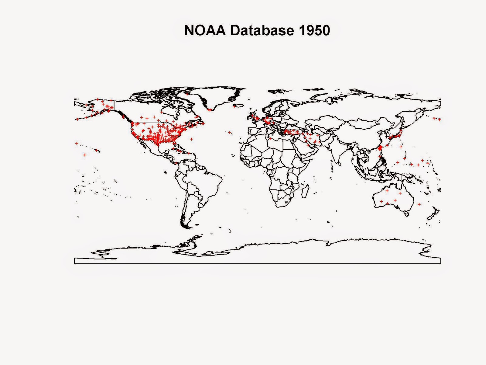
However, if we skip forward 10 years to 1950, the pictures changes. 

The second world war was just over and now we have weather stations all across countries that were highly involved in it. We have several stations in UK, Germany, Australia, Japan, Turkey, Palestine, Iran and Iraq.

A similar pattern can be seen if we take a look at the dataset available in 1960:

Here the striking addition are the numerous stations in Vietnam and surroundings. It is probably easy to understand the reason.

Sometimes we forget that our work can be used for good, but it can also be very useful in bad times!!

Here is the complete code to reproduce this experiment:

library(raster)
library(gstat)
library(XML)
library(plotrix)


setwd("D:/Wind Speed Co-Kriging - IPA Project")

#Extract Coordinates for each Station
coords.fwt <- read.fwf("ftp://ftp.ncdc.noaa.gov/pub/data/gsod/isd-history.txt",widths=c(6,1,5,1,38,7,1,8,9,8,1,8),sep=";",skip=21,fill=T)
coords <- data.frame(ID=paste(as.factor(coords.fwt[,1])),WBAN=paste(as.factor(coords.fwt[,3])),Lat=as.numeric(paste(coords.fwt$V6)),Lon=as.numeric(paste(coords.fwt$V8)))


#Download Measurements
year = 2013
dir.create(paste(getwd(),"/Data",sep=""))
download.file(paste("ftp://ftp.ncdc.noaa.gov/pub/data/gsod/",year,"/gsod_",year,".tar",sep=""),destfile=paste(getwd(),"/Data/","gsod_",year,".tar",sep=""),method="auto",mode="wb")
#Extract Measurements
dir.create(paste(getwd(),"/Data/Files",sep=""))
untar(paste(getwd(),"/Data/","gsod_",year,".tar",sep=""),exdir=paste(getwd(),"/Data/Files",sep=""))


#Create Data Frame
files <- list.files(paste(getwd(),"/Data/Files/",sep=""))

classes <- c(rep("factor",3),rep("numeric",14),rep("factor",3),rep("numeric",2))

t0 <- Sys.time()
station <- data.frame(Lat=numeric(),Lon=numeric(),TempC=numeric())
for(i in 1:length(files)){

data <- read.table(gzfile(paste(getwd(),"/Data/Files/",files[i],sep=""),open="rt"),sep="",header=F,skip=1,colClasses=classes)
if(paste(unique(data$V1))!=paste("999999")){
coords.sub <- coords[paste(coords$ID)==paste(unique(data$V1)),]

 if(nrow(data)>(365/2)){
  ST1 <- data.frame(TempC=(data$V4-32)/1.8,Tcount=data$V5)
  ST2 <- ST1[ST1$Tcount>12,]
  ST3 <- data.frame(Lat=coords.sub$Lat,Lon=coords.sub$Lon,TempC=round(mean(ST2$TempC,na.rm=T),2))
  station[i,] <- ST3
 }
} else {
coords.sub <- coords[paste(coords$WBAN)==paste(unique(data$V2)),]

 if(nrow(data)>(365/2)&coords.sub$Lat!=0&!is.na(coords.sub$Lat)){
  ST1 <- data.frame(TempC=(data$V4-32)/1.8,Tcount=data$V5)
  ST2 <- ST1[ST1$Tcount>12,]
  ST3 <- data.frame(Lat=coords.sub$Lat,Lon=coords.sub$Lon,TempC=round(mean(ST2$TempC,na.rm=T),2))
  station[i,] <- ST3
 }

}
print(i)
flush.console()
}
t1 <- Sys.time()
t1-t0

Temperature.data <- na.omit(station)
coordinates(Temperature.data)=~Lon+Lat

dir.create(paste(getwd(),"/Data/Polygons",sep=""))
download.file("http://thematicmapping.org/downloads/TM_WORLD_BORDERS_SIMPL-0.3.zip",destfile=paste(getwd(),"/Data/Polygons/","TM_WORLD_BORDERS_SIMPL-0.3.zip",sep=""))
unzip(paste(getwd(),"/Data/Polygons/","TM_WORLD_BORDERS_SIMPL-0.3.zip",sep=""),exdir=paste(getwd(),"/Data/Polygons",sep=""))
polygons <- shapefile(paste(getwd(),"/Data/Polygons/","TM_WORLD_BORDERS_SIMPL-0.3.shp",sep=""))


jpeg(paste(getwd(),"/Data/",year,".jpg",sep=""),2000,1500,res=300)
plot(polygons,main=paste("NOAA Database ",year,sep=""))
points(Temperature.data,pch="+",cex=0.5,col=color.scale(Temperature.data$TempC,color.spec="hsv"))
dev.off()

World Point Grid

These days I am following a couple of master projects dealing with renewable energy potentials at the global scale. We wanted to try and compute these potential using only free data and see how far we could go.
For wind speed there are plenty of resources freely available on the web. In particular my students downloaded the daily averages from NOAA: http://gis.ncdc.noaa.gov/geoportal/catalog/search/resource/details.jsp?id=gov.noaa.ncdc%3AC00516

One of the problem they encountered was that obviously these data are available for discrete locations, where meteorological stations are located, and if we want to create a map out of them we need to use some form of estimation. The time was limited so we opted for one of the simplest out there, i.e. kriging. Using other form of estimations optimized for wind, like dispersion or other physical modelling would have been almost impossible to pull off at the global scale. These models need too much time, we are talking about month of computations for estimating wind speed in one single country.
Anyway, ETH is an ESRI development centre and therefore the students normally do their work in ArcGIS, this project was no exception. For this reason we used Geostatistical Analyst in ArcGIS for the interpolation. The process was fast considering that we were dealing with a global scale interpolation; even when we used two covariates and we tested co-kriging the entire process was completed in less that 10 minutes, more or less.
The problem is that the output of Geostatistical Analyst is a sort of contours raster, which cannot be directly used to export its value onto a point grid. In this project we were planning to work on a 1Km scale, meaning that we would have need a mean wind speed value for each point on a 1Km grid. In theory this can be done directly from ArcGIS, you can use the function "Create Fishnet" to create the point grid and then the prediction function in Geostatistical Analyst to estimate an interpolated value for each point in the grid. I said in theory because in practice creating a point grid for the whole world is almost impossible with standard PCs. In our students labs we have 4Gb of RAM in each PC and with that there is no way to do the create the grid. We also tried a sort of "raw parallellization", meaning that we used 10 PCs to create one small parts of the grid, then extract just the part that overlay with land (and exclude oceans). Even with this process (which is by no means practical, elegant or fast) we were unable to finish the process. Even 1/10 of the world grid is enough to fill 4Gb of RAM.
In the end we decided to work on a 10Km scale because we simply did not have time to try alternative routes. However, the whole thing make me think about possible ways of creating a point grid for the whole World in R. We could use the function spsample to create point grids using polygon shapefiles, but unless you have a ton of RAM there is no way of doing it in one go. So I thought about iterating through the country polygons, create small grid and export their coordinates in an external txt. Even this process did not work, as soon as the loop reached Argentina the process filled the 8Gb of RAM of my PC and it stopped.
The solution was the use of even smaller scale polygons. I downloaded the Natural Earth 1:10m cultural dataset with States and Provinces and iterated through that. The process takes quite a long time, using one CPU, but it can probably be parallelized. The final dimension of the file with just two columns with the coordinates is 4.8Gb. This can be used directly by loading it as an ff data.frame (read.table.ffdf) or by loading only small chucks of it in an iterative fashion once you need to use it for estimations.
The R script I created takes care of the whole process. It downloads the dataset from Natural Earth, excludes Antartica, which is too big, run the loop and saves a TXT file in the working directory.

This is my code, I hope it can help you somehow:

library(raster)
library(ff)


setwd("C:/")

download.file("http://www.naturalearthdata.com/http//www.naturalearthdata.com/download/10m/cultural/ne_10m_admin_1_states_provinces.zip",destfile="ne_10m_admin_1_states_provinces.zip")
unzip("ne_10m_admin_1_states_provinces.zip",exdir="StateProvinces")

setwd("C:/StateProvinces")

polygons <- shapefile(list.files(pattern=".shp"))
polygons <- polygons[! paste(polygons$name) %in% paste("Antarctica"),]

names(polygons)

i=1
while(i<=nrow(polygons)){
if(paste(polygons[i,]$name)!=paste("NA")){
 grids <- try(spsample(polygons[i,],cellsize=0.01,type="regular"))

 if(inherits(grids, "try-error"))
    {
      i = i+1
    } else {

 write.table(as.data.frame(grids),"Grid_1Km.txt",sep=" ",row.names=F,col.names=F,append=T)
 
 print(i)
 flush.console()
 i=i+1 }
} else { i = i+1 }
}

#file.remove("Grid_1Km.txt")

grid <- read.table.ffdf(file="Grid_1Km.txt",nrows=1000,sep=",")
names(grid)

R Object-oriented Programming - Book Review

I have been asked to review the book “R Object-oriented Programming” by Kelly Black, edited by Packt publishing (£14.45 for the E-Book, £27.99 for Print+E-Book).

The scope of the book is “to provide a resource for programming using the R language” and therefore it can be seen as a good and practical introduction to all the most commonly used part of R. The first 2 chapters deal with data type and data organization in R. They basically quickly review how to handle each type of data (such as integers, doubles) and how to organize them into R objects. The third chapter deals with reading data from files and save them. This chapter gives a pretty good introduction into reading and writing every sort of data, even binaries, and from a variety of sources, including from the web. Chapter 4 provides an introduction to R commands to generate random numbers, in particular it gives a thorough overview of the sample command. Chapters 5 and 6 give a good background into the use of R to manipulate string and time variables. Of particular interest throughout the book is the handling of data gathered from public source on the web. For these particular data skills in string manipulation become crucial both for handling web addresses and also to extract the actual data from the information returned by the server. For this reason I think this book does a good job in introducing these important aspect of the R language.

Chapter 7 introduces some basic programming concepts, such as if statements and loops. Chapters 8 and 9 provide a complete overview of the S3 and S4 classes and finally chapters 10 and 11 are two hands on examples on how to put together all the concepts learned in the book to solve very practical problems. In these example the reader will be guided towards the creation of powerful R programs to grade student and perform a Monte Carlo simulation.

The book is written in a very practical form, meaning that not much time is wasted explaining each function in details, readers can browse the help pages of each function for more details. This means that probably this book is not for newbies to programming languages. Most of the learning is done by exploring the lines of code provided and for this reason I think the best readers would be people familiar with a programming language, even though I do not think that readers necessarily needs some familiarity with R. However as stated on the website, the target for this book are beginners who wants to become more “fluent” with the language.

Overall, I think this book does a good of providing the reader with a strong and neat introduction to all the bits of coding required to become more comfortable writing advance scripts. For example, at the end of chapter 2 the author discuss the use of the apply set of commands. These are crucial milestone to be learned for every individual who wants to switch from a mundane use of R to a more advanced and rigorous use of the language. In my personal experience when I began using R I would often create very long script using lots of loops and if statements, which tends to greatly decrease the execution speed. As soon as I learned to master the apply set of commands I was able to reduce my code and crucially I was also able to substantially increase its executing speed. Personally I would have loved to have access to such a book back then! The use of web sources for data manipulation is also a very nice addition that as far as I know is not common in other introductory texts. Nowadays gathering data from the web has become the norm and therefore I think it is important to provide beginners with tools to handle these type of data.

The strength of this book however is in chapters 8 and 9, which provide an extensive introduction to the use of the classes S3 and S4. I think these two chapters alone would justify the price for buying it. As far as I know these concepts are generally not treated with the right attention in books for beginners. They may explain you that when you load a package then the functions you normally use, such as plot, may change their function and options. However, I never found an introductory book that provides such as exhaustive explanation of how to fully control these classes to create advance programs. Of particular interest are also the two examples provided in Chapters 10 and 11. These are practical exercises that put together all the concepts learned in the previous chapters with the purpose of creating R programs that can be easily implemented and share. Chapter 10 for example describe a neat and powerful way to create a new R program to grade students. In this chapter the reader will use all the basic programming concept learned during the course of the book and he/she will put them together for creating an R program to import grades from csv files, manipulate them and create summary statistics and plot.

In conclusion, I see a variety of uses for this book. Clearly it is targeted to post beginners who need a short way to unlock the full power of R for their daily statistical routines. However, this book does not loose its purpose after we learned to properly use the language. It is written in such a way that even for experienced R users it is a useful way to quickly look-up functions and methods that maybe they do not use very often. I sometimes forget how to use certain functions and having such a book on my office bookshelf will certainly help me in these frustrating situations. So I think it will become part of the set of references that future R user will use on a regular basis.