Saturday, 15 July 2017

Generalized Additive Models and Mixed-Effects in Agriculture

Introduction

In the previous post I explored the use of linear model in the forms most commonly used in agricultural research.
Clearly, when we are talking about linear models we are implicitly assuming that all relations between the dependent variable y and the predictors x are linear. In fact, in a linear model we could specify different shapes for the relation between y and x, for example by including polynomials (read for example: https://datascienceplus.com/fitting-polynomial-regression-r/). However, we can do that only in cases where we can clearly see a particular shape of the relation, for example quadratic. The problem is in many cases we can see from a scatterplot that we have a non-linear distribution of the points, but it is difficult to understand its form. Moreover, in a linear model the interpretation of polynomial coefficients become more difficult and this may decrease their usefulness.
An alternative approach is provided by Generalized Additive Models, which allows us to fit models with non-linear smoothers without specifying a particular shape a priori.

I will not go into much details about the theory behind GAMs. You can refer to these two books (freely available online) to know more:

Wood, S.N., 2017. Generalized additive models: an introduction with R. CRC press.
http://reseau-mexico.fr/sites/reseau-mexico.fr/files/igam.pdf

Crawley, M.J., 2012. The R book. John Wiley & Sons.
https://www.cs.upc.edu/~robert/teaching/estadistica/TheRBook.pdf


Some Background

As mentioned above, GAM models are more powerful that the other linear model we have seen in previous posts since they allow to include non-linear smoothers into the mix. In mathematical terms GAM solve the following equation:

It may seem like a complex equation, but actually it is pretty simple to understand. The first thing to notice is that with GAM we are not necessarily estimating the response directly, i.e. we are not modelling y. In fact, as with GLM we have the possibility to use link functions to model non-normal response variables (and thus perform poisson or logistic regression). Therefore, the term g(μ) is simply the transformation of y needed to "linearize" the model. When we are dealing with a normally distributed response this term is simply replace by y.
Now we can explore the second part of the equation, where we have two terms: the parametric and the non-parametric part. In GAM we can include all the parametric terms we can include in lm or glm, for example linear or polynomial terms. The second part is the non-parametric smoother that will be fitted automatically and it is the key point of GAMs.
To better understand the difference between the two parts of the equation we can explore an example. Let's say we have a response variable (normally distributed) and two predictors x1 and x2. We look at the data and we observe a clear linear relation between x1 and y, but a complex curvilinear pattern between x2 and y. Because of this we decide to fit a generalized additive model that in this particular case will take the following equation:

Since y is normal we do not need the link function g(). Then we are modelling x1 as a linear model with intercept beta zero and coefficient beta one. However, since we observed a curvilinear relation between x2 and y we also including a non-parametric smoothing function to model x2.


Practical Example

In this tutorial we will work once again with the package agridat so that we can work directly with real data in agriculture. Other packages we will use are ggplot2, moments, pscl and MuMIn:

 library(agridat)  
 library(ggplot2)  
 library(moments)  
 library(pscl)  
 library(MuMIn)  

In R there are two packages to fit generalized additive models, I will talk about the package mgcv. For an overview of GAMs from the package gam you can refer to this post: https://datascienceplus.com/generalized-additive-models/

The first thing we need to do is install the package mgcv:

 install.packages("mgcv")  
 library(mgcv)  

Now we can load once again the package lasrosas.corn with measures of yield based on nitrogen treatments, plus topographic position and brightness value (for more info please take a look at my previous post: Linear Models (lm, ANOVA and ANCOVA) in Agriculture). Then we can use the function pairs to plot all variable in scatterplots, colored by topographic position:

 dat = lasrosas.corn  
 attach(dat)  
 pairs(dat[,4:9], lower.panel = NULL, col=topo)  

This produces the following image:


In the previous post we only fitted linear models to these data, and therefore the relations between yield and all other predictors were always modelled as lines. However, if we look at the scatterplot between yield and bv, we can clearly see a pattern that does not really look linear, with some blue dots that deviates from the main cloud. If these blue dots were not present we would be happy in modelling this relation as linear. In fact we can prove that by only focusing on this plot and removing the level W from topo:

 par(mfrow=c(1,2))  
 plot(yield ~ bv, pch=20, data=dat, xlim=c(100,220))  
 plot(yield ~ bv, pch=20, data=dat[dat$topo!="W",], xlim=c(100,220))  

which creates the following plot:
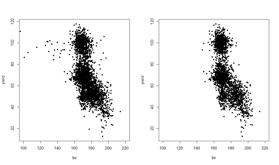
From this plot it is clear that the level W is an anomaly compared to the rest of the dataset. However, even removing this from the dataset does not really produce a linear pattern, but more a quadratic one. For this reason, it may be that if we want to obtain the best possible results in terms of modelling yield we would need to split the data by topographic position. However, for this post we are not interested in this, but only in showing the use of GAMs. Therefore, we will keep all levels of topo and then try to model the relation between yield and topo with a non-parametric smoother.

 mod.lm = lm(yield ~ bv)  
 mod.quad = lm(yield ~ bv + I(bv^2))  
 mod.gam = gam(yield ~ s(bv), data=dat)  

Here we are testing three models: standard linear model, a linear model with a quadratic term and finally a GAM. We do that because clearly we are not sure which model is the best and we want to make sure we do not overfit our data.
We can compare these models in the same way we explored in previous posts: by calculating the Akaike Information Criterion (AIC) and with an F test.

 > AIC(mod.lm, mod.quad, mod.gam)  
         df   AIC  
 mod.lm  3.000000 29005.32  
 mod.quad 4.000000 28924.18  
 mod.gam 7.738304 28853.72  
 > anova(mod.lm, mod.quad, mod.gam, test="F")  
 Analysis of Variance Table  
 Model 1: yield ~ bv  
 Model 2: yield ~ bv + I(bv^2)  
 Model 3: yield ~ s(bv)  
  Res.Df  RSS   Df Sum of Sq   F  Pr(>F)    
 1 3441.0 917043                     
 2 3440.0 895165 1.0000   21879 85.908 < 2.2e-16 ***  
 3 3436.3 875130 3.7383   20034 21.043 3.305e-16 ***  
 ---  
 Signif. codes: 0 ‘***’ 0.001 ‘**’ 0.01 ‘*’ 0.05 ‘.’ 0.1 ‘ ’ 1  

The AIC suggests that the GAM is slightly more accurate that the other two, even with more degrees of freedom. The F test again results in significant difference between models, thus suggesting that we should use the more complex model.

We can look at the difference in fitting of the three models graphically first using the standard plotting function and then with ggplot2:

 plot(yield ~ bv, pch=20)  
 abline(mod.lm,col="blue",lwd=2)  
 lines(50:250,predict(mod.gam, newdata=data.frame(bv=50:250)),col="red",lwd=2)  
 lines(50:250,predict(mod.quad, newdata=data.frame(bv=50:250)),col="green",lwd=2)  

This produces the following image:


The same can be achieved with ggplot2:

 ggplot(data=dat, aes(x=bv, y=yield)) +  
      geom_point(aes(col=dat$topo))  +  
      geom_smooth(method = "lm", se = F, col="red")+  
      geom_smooth(method="gam", formula=y~s(x), se = F, col="blue") +  
      stat_smooth(method="lm", formula=yield~x+I(x^2),se = F, col="green")  

which produces the following:


This second image is even more informative because when we decide to use a categorical variable to color the dots, ggplot2 automatically creates a legend for it, so we know which level causes the shift in the data (i.e. W).

As you can see all of these lines do not really fit the data perfectly, since the large cloud around 100 in yield and 180 in bv is not considered. However, the blue line of the non-parametric smoother seems to better catch the violet dots on the left and also bends when reaches the cloud, mimicking the quadratic behavior we observed before.

With GAM we can still use the function summary to look at the model in details:

 > summary(mod.gam)  
 Family: gaussian   
 Link function: identity   
 Formula:  
 yield ~ s(bv)  
 Parametric coefficients:  
       Estimate Std. Error t value Pr(>|t|)    
 (Intercept)  69.828   0.272  256.7  <2e-16 ***  
 ---  
 Signif. codes: 0 ‘***’ 0.001 ‘**’ 0.01 ‘*’ 0.05 ‘.’ 0.1 ‘ ’ 1  
 Approximate significance of smooth terms:  
     edf Ref.df   F p-value    
 s(bv) 5.738 6.919 270.7 <2e-16 ***  
 ---  
 Signif. codes: 0 ‘***’ 0.001 ‘**’ 0.01 ‘*’ 0.05 ‘.’ 0.1 ‘ ’ 1  
 R-sq.(adj) = 0.353  Deviance explained = 35.4%  
 GCV = 255.17 Scale est. = 254.68  n = 3443  

The interpretation is similar to linear models, and probably a bit easier that with GLM since in GAM we also have an R Squared directly from the summary output. As you can see the smooth term is highly significant and we can see its estimated degrees of freedom (around 6) and its F and p values. At the bottom of the output we see a numerical value for GCV, which stands for Generalized Cross Validation Score. This is what the model tries to reduce by default and it is given by the equation below:


where D is the deviance, n is the number of samples, and df the effective degrees of freedom of the model. for more info please refer to Wood's book. I read on-line in an answer on StackOverflow that GCV may produce underfitting, I am not completely sure about this because I have not found any mention of it on official documentations. However, just in case later on I will show you how to fit the smoother with REML, which according to StackOverflow should solve the issue with underfitting.

Include more parameters


Now that we have a general idea about what function to fit for bv we can add more predictors and try to create a more accurate model.

 > #Include more predictors  
 > mod.lm = lm(yield ~ nitro + nf + topo + bv)  
 > mod.gam = gam(yield ~ nitro + nf + topo + s(bv), data=dat)  
 >   
 > #Comparison R Squared  
 > summary(mod.lm)$adj.r.squared  
 [1] 0.5211237  
 > summary(mod.gam)$r.sq  
 [1] 0.5292042  

In the code above we are comparing two models with all of the predictors we have in the datasets. As you can see there is not much difference in the two models in terms of R Squared, so both model are able to explain pretty much the same level of variation in yield.

However, as you remember from above, we clearly noticed changes in bv depending on topo, and we also noticed that if we exclude certain topographic categories the behavior of the curve would probably change. We can include this new hypothesis in the model by using the option by within s, to fit a non-parametric smoother to each topographic factor individually.

 > mod.gam2 = gam(yield ~ nitro + nf * topo + s(bv, by=topo), data=dat)  
 >   
 > summary(mod.gam2)$r.sq  
 [1] 0.5612617  

As you can see if we fit a curve to each subset of the plot above we can increase the R Squared, and therefore explain more variation in yield.
We can further explore the difference in models with function AIC and anova, as we've seen in previous posts:

 > AIC(mod.lm, mod.gam, mod.gam2)  
         df   AIC  
 mod.lm  12.00000 27815.23  
 mod.gam 18.60852 27763.83  
 mod.gam2 42.22616 27548.63  
 >   
 > #F test  
 > anova(mod.lm, mod.gam, mod.gam2, test="F")  
 Analysis of Variance Table  
 Model 1: yield ~ nitro + nf + topo + bv  
 Model 2: yield ~ nitro + nf + topo + s(bv)  
 Model 3: yield ~ nitro + nf * topo + s(bv, by = topo)  
  Res.Df  RSS   Df Sum of Sq   F  Pr(>F)    
 1 3432.0 645661                      
 2 3425.4 633656 6.6085   12005 10.525 1.512e-12 ***  
 3 3401.8 587151 23.6176   46505 11.408 < 2.2e-16 ***  
 ---  
 Signif. codes: 0 ‘***’ 0.001 ‘**’ 0.01 ‘*’ 0.05 ‘.’ 0.1 ‘ ’ 1  

The AIC is lower for mod.gam2, and the F test suggest it is significantly different from the other, meaning that we should use the more complex model.

Another way of assessing the accuracy of our two models would be to use some diagnostic plots. Let's start with the model with a non-parametric smoother fitted to the whole datasets (mod.gam):

 plot(mod.gam, all.terms=F, residuals=T, pch=20)  

which produce the following image:

This plot can be interpreted exactly like the fitted vs. residuals plot we produced for the post about linear model (see here: Linear Models (lm, ANOVA and ANCOVA) in Agriculture). For the model to be good we would expect this line to be horizontal and the spread to be more or less homogeneous (this is except when dealing with time-series, please see here: Analyzing-double-seasonal-time-series-with-GAM-in-R). However, this is clearly not the case and this strongly suggest our model is not a good one.
Now let's take a look at the same plot for mod.gam2, the one where we fitted a curve for each level of topo:

 par(mfrow=c(2,2))  
 plot(mod.gam2, all.terms=F, residuals=T, pch=20, page=1)  

In this case we need to use the function par to create 4 sub-plots within the plotting window. This is because now the model fits a curve for each of the four categories in topo, so four plots will be created.

The result is clearly much better. All lines are more or less horizontal, even tough in some case the spread of the confidence intervals in uneven. However, this model is clearly a step forward in term of accuracy compared to mod.gam.

Another useful function for producing diagnostic plots is gam.check:

 par(mfrow=c(2,2))  
 gam.check(mod.gam2)  

which creates the following:


This shows similar plots to what we see in the previous post about linear models. Again we are aiming at normally distributed residuals. Moreover, the plot residuals vs. fitted should show a cloud centered around 0 and with more or less equal variance throughout the range of fitted values, which is approximately what we see here.


Changing Parameters

The function s, used to fit non-parametric smoother, can take a series of option that changes it behavior. We will now look at some of them:

 mod.gam1 = gam(yield ~ s(bv), data=dat)  
 mod.gam2 = gam(yield ~ s(bv), data=dat, gamma=1.4)   
 mod.gam3 = gam(yield ~ s(bv), data=dat, method="REML")  
 mod.gam4 = gam(yield ~ s(bv, bs="cr"), data=dat) #All options for bs at help(smooth.terms)  
 mod.gam5 = gam(yield ~ s(bv, bs="ps"), data=dat)  
 mod.gam6 = gam(yield ~ s(bv, k=2), data=dat)  

The first line is the standard use, without any option and we will use it just for comparison. The second call (mod.gam2) changes the gamma, which increases the "penalty" per increment in degree of freedom. Its default value is 1, but Wood suggest that increasing it to 1.4 can reduce over-fitting (Pag. 227 of Wood's book, link on top of the page). The third model fits the GAM using REML instead of the standard GCV score, which should provide a more robust fitting. The fourth and fifth models use the option bs within the function s to change the way the curve is fitted. In mod.gam4, cr stands for cubic regression spline, while in mod.gam5 ps stands for P-Splines. There are several options available for bs and you can look at them with help(smooth.terms). Each of these option comes with advantages and disadvantages; to know more about this topic you can read pag. 222 from Wood's book.
The final model (mod.gam6) changes the dimension of the curve, with which we can select the maximum degrees of freedom (default value is 10). In this case we are basically telling R to fit a quadratic curve.
We can plot all the lines generated from the models above to have an idea of individual impacts:

 plot(yield ~ bv, pch=20)  
 lines(50:250,predict(mod.gam1, newdata=data.frame(bv=50:250)),col="blue",lwd=2)  
 lines(50:250,predict(mod.gam2, newdata=data.frame(bv=50:250)),col="red",lwd=2)  
 lines(50:250,predict(mod.gam3, newdata=data.frame(bv=50:250)),col="green",lwd=2)  
 lines(50:250,predict(mod.gam4, newdata=data.frame(bv=50:250)),col="yellow",lwd=2)  
 lines(50:250,predict(mod.gam5, newdata=data.frame(bv=50:250)),col="orange",lwd=2)  
 lines(50:250,predict(mod.gam6, newdata=data.frame(bv=50:250)),col="violet",lwd=2)  


As you can see the violet line is basically a quadratic curve, while the rest are quite complex in shape. In particular, the orange line created with P-splines looks like is overfitting the data, while the other look generally the same.


Count Data - Poisson Regression

GAM can be used with all the distributions and link function we have explored for GLM (Generalized Linear Models). To explore this we are going to use another dataset from the package agridat: named mead.cauliflower. This dataset presents leaves for cauliflower plants at different times.

 dat = mead.cauliflower  
 str(dat)  
 attach(dat)  
 pairs(dat, lower.panel = NULL)   

From the pairs plot it seems that a linear model would probably describe the relation between leaves and the variable degdays pretty well. However, since we are talking about GAMs we will try to fit a generalized additive model and see how it compares to that standard GLM.

 pois.glm = glm(leaves ~ year + degdays, data=dat, family=c("poisson"))  
 pois.gam = gam(leaves ~ year + s(degdays), data=dat, family=c("poisson"))  

as you can see there are only minor differences in the syntax between the two lines. We are still using the option family to specify that we want the poisson distribution for the error term, plus the log link (used by default so we do not need to specify it).
To compare the model we can again use AIC and anova:

 > AIC(pois.glm, pois.gam)  
         df   AIC  
 pois.glm 3.000000 101.4505  
 pois.gam 3.431062 101.1504  
 >   
 > anova(pois.glm, pois.gam)  
 Analysis of Deviance Table  
 Model 1: leaves ~ year + degdays  
 Model 2: leaves ~ year + s(degdays)  
  Resid. Df Resid. Dev   Df Deviance  
 1  11.000   6.0593           
 2  10.569   4.8970 0.43106  1.1623  

Both results suggest that in fact a GAM for this dataset is not needed, since it is only slightly different from the GLM model. We could also compare the R Squared of the two models, using the function to compute it for GLM we tested in the previous post:

 > pR2(pois.glm)  
      llh   llhNull      G2   McFadden     r2ML     r2CU   
  -47.7252627 -132.3402086 169.2298918  0.6393744  0.9999944  0.9999944   
 > r.squaredLR(pois.glm)  
 [1] 0.9999944  
 attr(,"adj.r.squared")  
 [1] 0.9999944  
 >   
 > summary(pois.gam)$r.sq  
 [1] 0.9663474  

For overdispersed data we have the option to use both the quasipoisson and the negative binomial distributions:

 pois.gam.quasi = gam(leaves ~ year + s(degdays), data=dat, family=c("quasipoisson"))  
 pois.gam.nb = gam(leaves ~ year + s(degdays), data=dat, family=nb())  

For more info about the use of the negative binomial please look at this article:
GAMs with the negative binomial distribution


Logistic Regression

Since we can use of the families we have in GLMs we can also use GAM with binary data, the syntax again is very similar to what we used for GLM:

 dat = johnson.blight  
 str(dat)  
 attach(dat)  
 logit.glm = glm(blight ~ rain.am + rain.ja + precip.m, data=dat, family=binomial)  
 logit.gam = gam(blight ~ s(rain.am, rain.ja,k=5) + s(precip.m), data=dat, family=binomial)  

As you can see we are using an interaction between rain.am and rain.ja in the model, plus another smooth curve fitted only to precip.m.
We can compare the two models as follows:

 > anova(logit.glm, logit.gam, test="Chi")  
 Analysis of Deviance Table  
 Model 1: blight ~ rain.am + rain.ja + precip.m  
 Model 2: blight ~ s(rain.am, rain.ja, k = 5) + s(precip.m)  
  Resid. Df Resid. Dev     Df  Deviance Pr(>Chi)    
 1    21   20.029                    
 2    21   20.029 1.0222e-05 3.4208e-06 6.492e-05 ***  
 ---  
 Signif. codes: 0 ‘***’ 0.001 ‘**’ 0.01 ‘*’ 0.05 ‘.’ 0.1 ‘ ’ 1  
 >   
 > AIC(logit.glm, logit.gam)  
         df   AIC  
 logit.glm 4.00000 28.02893  
 logit.gam 4.00001 28.02895  

Despite the identical AIC values, the fact that the anova test is significant suggests we should use the more complex model, i.e. the GAM.

In the package mgcv there is also a function dedicated to the visualization of the curve on the response variable:

 vis.gam(logit.gam, view=c("rain.am", "rain.ja"), type="response")  

this creates the following 3D plot:

This shows the response on the z axis and the two variables associated in the interaction. Since this plot is a bit difficult to interpret we can also plot is as contours:

 vis.gam(logit.gam, view=c("rain.am", "rain.ja"), type="response", plot.type="contour")  
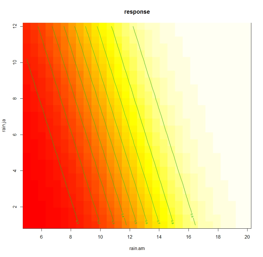
This allows to determine the changes in Leaves dependent only from the interaction between rain.am and rain.ja.


Generalized Additive Mixed Effects Models

In the package mgcv there is the function gamm, which allows fitting generalized additive mixed effects model, with a syntax taken from the package nlme. However, compared to what we see in the post about Mixed-Effects Models there are some changes we need to make.
Let's focus again on the dataset lasrosas.corn, which has a column year that we can consider as a possible source of additional random variation. The code below imports the dataset and then transform the variable year from numeric to factorial:

 dat = lasrosas.corn  
 dat$year = as.factor(paste(dat$year))  

We will start by looking at a random intercept model. If this was not a GAM with mixed effects, but a simpler linear mixed effects model, the code to fit it would be the following:

 LME = lme(yield ~ nitro + nf + topo + bv, data=dat, random=~1|year)  

This is probably the same line of code we used in the previous post. In the package nlme this same model can be fitted using a list as input for the option random. Look at the code below:

 LME1 = lme(yield ~ nitro + nf + topo + bv, data=dat, random=list(year=~1))   

Here in the list we are creating a new value year, which takes a value of ~1, indicating that its random effect applies only to the intercept.
We can use the anova function to see that LME and LME2 are in fact the same model:

 > anova(LME, LME1)  
    Model df   AIC   BIC  logLik  
 LME   1 13 27138.22 27218.05 -13556.11  
 LME1   2 13 27138.22 27218.05 -13556.11  

I showed you this alternative syntax with list because in gamm this is the only syntax we can use. So for fitting a GAM with random intercept for year we should use the following code:

 gam.ME = gamm(yield ~ nitro + nf + topo + s(bv), data=dat, random=list(year=~1))  

The object gam.ME is a list with two component, a mixed effect mode and a GAM. To check their summaries we need to use two lines:

 summary(gam.ME[[1]])  
 summary(gam.ME[[2]])  


Now we can see the code to fit a random slope and intercept model. gain we need to use the syntax with a list:

 gam.ME2 = gamm(yield ~ nitro + nf + topo + s(bv), data=dat, random=list(year=~1, year=~nf))  

Here we are including two random effects, one for just the intercept (year=~1) and another for random slope and intercept for each level of nf (year=~nf).

Monday, 10 July 2017

Assessing the Accuracy of our models (R Squared, Adjusted R Squared, RMSE, MAE, AIC)

Assessing the accuracy of our model

There are several ways to check the accuracy of our models, some are printed directly in R within the summary output, others are just as easy to calculate with specific functions. Please take a look at my previous post for more info on the code.


R Squared

This is probably the most commonly used statistics and allows us to understand the percentage of variance in the target variable explained by the model. It can be computed as a ratio of the regression sum of squares and the total sum of squares. This is one of the standard measures of accuracy that R prints out, through the function summary, for linear models and ANOVAs.


Adjusted R Squared

This is a form of R-squared that is adjusted for the number of predictors in the model. It can be computed as follows:

Where R2 is the R squared of the model, n is the sample size and p is the number of terms (or predictors) in the model. This index is extremely useful to determine whether our model is overfitting the data. This happens particularly when the sample size is small, in such cases if we fill the model with more predictors we may end up increasing the R squared simply because the model starts adapting to the noise (or random error) and not properly describing the data. It is a generally good indication if the adjusted R squared is similar to the standard R squared.


Root Mean Squared Deviation or Root Mean Squared Error

The previous indexes measure the amount of variance in the target variable that can be explained by our model. This is a good indication but in some cases we are more interested in quantifying the error in the same measuring unit of the variable. In such cases we need to compute indexes that average the residuals of the model. The problem is residuals are both positive and negative and their distribution should be fairly symmetrical (this is actually one of the assumptions in most linear models, so if this is not the case we should be worried). This means that their average will always be zero. So we need to find other indexes to quantify the average residuals, for example by averaging the squared residuals:

This is the square root of the mean of the squared residuals, with Yhat_t being the estimated value at point t, Y_t being the observed value in t and n being the sample size. The RMSE has the same measuring unit of the variable y.


Mean Squared Deviation or Mean Squared Error

This is simply the numerator of the previous equation, but it is not used often. The issue with both the RMSE and the MSE is that, since they square the residuals, they tend to be more affected by extreme values. This means that even if our model explains the large majority of the variation in the data very well, with few exceptions; these exceptions will inflate the value of RMSE if the discrepancy between observed and predicted is large. Since this large residuals may be caused by potential outliers, this issue may cause overestimation of the error.


Mean Absolute Deviation or Mean Absolute Error

To solve the problem with potential outliers, we can use the mean absolute error, where we average the absolute value of the residuals:
This index is more robust against large residuals. Since RMSE is still widely used, even though its problems are well known, it is always better to calculate and present both in a research paper.


Akaike Information Criterion

This is another popular index we have used in previous posts to compare different models. It is very popular because it corrects the RMSE for the number of predictors in the model, thus allowing to account for overfitting. It can be simply computed as follows:


Where again p is the number of terms in the model.

Linear Mixed Effects Models in Agriculture

This post was originally part of my previous post about linear models. However, I later decided to split it into several texts because it was effectively too long and complex to navigate.
If you struggle to follow the code in this page please refer to this post (for example for the necessary packages): Linear Models (lm, ANOVA and ANCOVA) in Agriculture


Linear Mixed-Effects Models

This class of models is used to account for more than one source of random variation. For example, assume we have a dataset where we are trying to model yield as a function of nitrogen levels. However, the data were collected in many different farms. In this case, each farm would need to be consider a cluster and the model would need to take this clustering into account. Another common set of experiments where linear mixed-effects models are used is repeated measures, where time provides an additional source of correlation between measures. For these models we do not need to worry about the assumptions from previous models, since these are very robust against all of them. For example, for unbalanced design with blocking, probably these methods should be used instead of the standard ANOVA.

At the beginning on this tutorial we explored the equation that supports linear model:


This equation can be divided into two components, the fixed and random effects. For fixed effect we refer to those variables we are using to explain the model. These may be factorial (in ANOVA), continuous or a mixed of the two (ANCOVA) and they can also be the blocks used in our design. The other component in the equation is the random effect, which provides a level of uncertainty that it is difficult to account for in the model. For example, when we work with yield we might see differences between plants grown from similar soils and conditions. These may be related to the seeds or to other factors and are part of the within-subject variation that we cannot explain.

There are times however where in the data there are multiple sources of random variation. For example, data may be clustered in separate fields or separate farms. This will provide an additional source of random variation that needs to be taken into account in the model. To do so the standard equation can be amended in the following way:


This is referred to as a random intercept model, where the random variation is split into a cluster specific variation u and the standard error term. Effectively, this model assumes that each cluster will only have an effect on the slope of the linear model. In other word, we assume that data collected at different farm will have the same correlation pattern but will be shifted, see image below (source: Mixed Models):


A more complex form, that is normally used for repeated measures is the random slope and intercept model:


Where we add a new source of random variation v related to time T. In this case we assume that the random variation happends not only by changing the intercept of the linear model, but also its slope. The image below from the same website should again clarify things:


As a general rule we can use plotting to determine if and what random effects to use for modelling our data. In the examples above, a simple xy plot with colour would provide a lot of information. Alternatively, we could use the plotting method with ggplot2 and the function facet_wrap to divide our scatterplots by factors and see if there are changes only in intercept or also slope.

Random Intercept Model for Clustered Data

In the following examples we will use the function lme in the package nlme, so please install and/or load the package first. For this example we are using the same dataset lasrosas.corn from package agridat we used in the previous post Linear Models in Agriculture

Just to explain the syntax to use linear mixed-effects model in R for cluster data, we will assume that the factorial variable rep in our dataset describes some clusters. To fit a mixed-effects model we are going to use the function lme from the package nlme. This function can work with unbalanced designs:

 lme1 = lme(yield ~ nf + bv * topo, random= ~1|rep, data=dat)  

The syntax is very similar to all the models we fitted before, with a general formula describing our target variable yield and all the treatments, which are the fixed effects of the model. Then we have the option random, which allows us to include an additional random component for the clustering factor rep. In this case the ~1 indicates that the random effect will be associated with the intercept.

Once again we can use the function summary to explore our results:

 > summary(lme1)  
 Linear mixed-effects model fit by REML  
  Data: dat   
     AIC   BIC  logLik  
  27648.36 27740.46 -13809.18  
   
 Random effects:  
  Formula: ~1 | rep  
     (Intercept) Residual  
 StdDev:  0.798407 13.3573  
   
 Fixed effects: yield ~ nf + bv * topo   
         Value Std.Error  DF  t-value p-value  
 (Intercept) 327.3304 14.782524 3428 22.143068    0  
 nfN1      3.9643 0.788049 3428  5.030561    0  
 nfN2      5.2340 0.790104 3428  6.624449    0  
 nfN3      5.4498 0.789084 3428  6.906496    0  
 nfN4      7.5286 0.789551 3428  9.535320    0  
 nfN5      7.7254 0.789111 3428  9.789976    0  
 bv      -1.4685 0.085507 3428 -17.173569    0  
 topoHT   -233.3675 17.143956 3428 -13.612232    0  
 topoLO   -251.9750 20.967003 3428 -12.017693    0  
 topoW    -146.4066 16.968453 3428 -8.628162    0  
 bv:topoHT   1.1945 0.097696 3428 12.226279    0  
 bv:topoLO   1.4961 0.123424 3428 12.121624    0  
 bv:topoW    0.7873 0.097865 3428  8.044485    0  
   

We can also use the function Anova to display the ANOVA table:

 > Anova(lme2, type=c("III"))  
 Analysis of Deviance Table (Type III tests)  
   
 Response: yield  
        Chisq Df Pr(>Chisq)    
 (Intercept) 752.25 1 < 2.2e-16 ***  
 nf     155.57 5 < 2.2e-16 ***  
 bv     291.49 1 < 2.2e-16 ***  
 topo    236.52 3 < 2.2e-16 ***  
 year    797.13 1 < 2.2e-16 ***  
 bv:topo   210.38 3 < 2.2e-16 ***  
 ---  
 Signif. codes: 0 ‘***’ 0.001 ‘**’ 0.01 ‘*’ 0.05 ‘.’ 0.1 ‘ ’ 1  
   

We might be interested in understanding if fitting a more complex model provides any advantage in terms of accuracy, compared with a model where no additional random effect is included. To do so we can compare this new model with mod6, which we created with the gls function and includes the same treatment structure.  We can do that with the function anova , specifying both models:

 > anova(lme1, mod6)  
    Model df   AIC   BIC  logLik  Test L.Ratio p-value  
 lme1   1 15 27648.36 27740.46 -13809.18              
 mod6   2 14 27651.21 27737.18 -13811.61 1 vs 2 4.857329 0.0275  
   

As you can see there is a decrease in AIC for the model fitted with lme, and the difference is significant (p-value below 0.05). Therefore this new model where clustering is accounted for is better than the one without an additional random effect, even though only slightly. In this case we would need to decide if fitting a more complex model (which is probably more difficult to explain to readers) is the best way.

Another way to assess the accuracy of GLS and Mixed Effects Models is through the use of pseudo R squared, which are indexes that can be interpreted as the normal R-Squared but calculated in different ways, since in these more complex models we do not calculate the sum of squares.
There are two important functions for this, both included in the package MuMIn:

 library(MuMIn)  
 > r.squaredLR(mod6)  
 [1] 0.5469906  
 attr(,"adj.r.squared")  
 [1] 0.5470721  
 > r.squaredGLMM(lme1)  
    R2m    R2c   
 0.5459845 0.5476009   

The first function r.squaredLR can be used for GLS models and provides both and R-Squared and an Adjusted R-Squared. The second function, r.squaredGLMM, is specific for mixed-effects models and provides two measures: R2m and R2c. The first reports the R2 of the model with just fixed effects, while the second the R squared of the full model.
In this case we can see again that the R squared are similar between models, and most importantly R2c is only slightly different compared to R2m, which means that including random effects does not improve the accuracy.

Random Intercept and Slope for repeated measures

If we collected data at several time steps we are looking at a repeated measures analysis, which is most cases can be treated as mixed random slope and intercept model. Again, we cannot just assume that because we have collected data over time we have a random slope and intercept, we always need to do some plotting first and take a closer look at our data. In cases like this where we are dealing with a factorial variable, we may be forced to rely on barcharts, divided by years. In such cases it may be difficult to understand whether we need a model this complex. So it may be that the only way is to just compare different models with anova (this function can be used with more than 2 models if needed).

The code to create such a model is the following:

 lme2 = lme(yield ~ nf + bv * topo + year, random= ~year|rep, data=dat)  
   
 summary(lme2)  
   
 Anova(lme2, type=c("III"))  
   

The syntax is very similar to what we wrote before, except that now the random component includes both time and clusters. Again we can use summary to get more info about the model. We can also use again the function anova to compare this with the previous model:

 > anova(lme1, lme2)  
    Model df   AIC   BIC  logLik  Test L.Ratio p-value  
 lme1   1 15 27648.36 27740.46 -13809.18              
 lme2   2 18 26938.83 27049.35 -13451.42 1 vs 2 715.5247 <.0001  
 Warning message:  
 In anova.lme(lme1, lme2) :  
  fitted objects with different fixed effects. REML comparisons are not meaningful.  
   

From this output it is clear that the new model is better that the one before and their difference in highly significant. If this happens it is generally better to adopt the more complex model.

We can extract only the effects for the random components using the function ranef:

 > ranef(lme2)  
   (Intercept)     year  
 R1 -0.3468601 -1.189799e-07  
 R2 -0.5681688 -1.973702e-07  
 R3  0.9150289 3.163501e-07   
   

This tells us the changes in yield for each cluster and time step.

We can also do the same for the fixed effects, and this will return the coefficients of the model:

 > fixef(lme2)  
  (Intercept)     nfN1     nfN2     nfN3     nfN4   
 -1.133614e+04 3.918006e+00 5.132136e+00 5.368513e+00 7.464542e+00   
      nfN5      bv    topoHT    topoLO     topoW   
  7.639337e+00 -1.318391e+00 -2.049979e+02 -2.321431e+02 -1.136168e+02   
      year   bv:topoHT   bv:topoLO   bv:topoW   
  5.818826e+00 1.027686e+00 1.383705e+00 5.998379e-01   
   

To have an idea of their confidence interval we can use the function intervals (package nlme):

 > intervals(lme2, which = "fixed")  
 Approximate 95% confidence intervals  
   
  Fixed effects:  
           lower     est.     upper  
 (Intercept) -1.214651e+04 -1.133614e+04 -1.052576e+04  
 nfN1     2.526139e+00 3.918006e+00 5.309873e+00  
 nfN2     3.736625e+00 5.132136e+00 6.527648e+00  
 nfN3     3.974809e+00 5.368513e+00 6.762216e+00  
 nfN4     6.070018e+00 7.464542e+00 8.859065e+00  
 nfN5     6.245584e+00 7.639337e+00 9.033089e+00  
 bv     -1.469793e+00 -1.318391e+00 -1.166989e+00  
 topoHT   -2.353450e+02 -2.049979e+02 -1.746508e+02  
 topoLO   -2.692026e+02 -2.321431e+02 -1.950836e+02  
 topoW    -1.436741e+02 -1.136168e+02 -8.355954e+01  
 year     5.414742e+00 5.818826e+00 6.222911e+00  
 bv:topoHT  8.547273e-01 1.027686e+00 1.200644e+00  
 bv:topoLO  1.165563e+00 1.383705e+00 1.601846e+00  
 bv:topoW   4.264933e-01 5.998379e-01 7.731826e-01  
 attr(,"label")  
 [1] "Fixed effects:"   


Syntax with lme4

Another popular package to perform mixed-effects models we could also use the package lme4 and the function lmer.
For example, to fit the model with random intercept (what we called lme1) we would use the following syntax in lme4:

 > lmer1 = lmer(yield ~ nf + bv * topo + (1|rep), data=dat)  
 >   
 > summary(lmer1)  
 Linear mixed model fit by REML ['lmerMod']  
 Formula: yield ~ nf + bv * topo + (1 | rep)  
   Data: dat  
 REML criterion at convergence: 27618.4  
 Scaled residuals:   
   Min   1Q Median   3Q   Max   
 -3.4267 -0.7767 -0.1109 0.7196 3.6892   
 Random effects:  
  Groups  Name    Variance Std.Dev.  
  rep   (Intercept)  0.6375 0.7984   
  Residual       178.4174 13.3573   
 Number of obs: 3443, groups: rep, 3  
 Fixed effects:  
        Estimate Std. Error t value  
 (Intercept) 327.33043  14.78252 22.143  
 nfN1      3.96433  0.78805  5.031  
 nfN2      5.23400  0.79010  6.624  
 nfN3      5.44980  0.78908  6.906  
 nfN4      7.52862  0.78955  9.535  
 nfN5      7.72537  0.78911  9.790  
 bv      -1.46846  0.08551 -17.174  
 topoHT   -233.36750  17.14396 -13.612  
 topoLO   -251.97500  20.96700 -12.018  
 topoW    -146.40655  16.96845 -8.628  
 bv:topoHT   1.19446  0.09770 12.226  
 bv:topoLO   1.49609  0.12342 12.122  
 bv:topoW    0.78727  0.09786  8.044  
 Correlation matrix not shown by default, as p = 13 > 12.  
 Use print(x, correlation=TRUE) or  
      vcov(x)     if you need it  

There are several differences between nlme and lme4 and I am not sure which is actually better. What I found is that probably lme4 is the most popular, but nlme is used for example to fit generalized addictive mixed effects models in the package mgcv. For this reason probably the best thing would be to know how to use both packages.

As you can see from the summary above, in this table there are no p-values, so it is a bit difficult to know which levels are significant for the model. We can solve this by installing and/or loading the package lmerTest. If we load lmerTest and run again the same function we would obtain the following summary table:

 > lmer1 = lmer(yield ~ nf + bv * topo + (1|rep), data=dat)  
 >   
 > summary(lmer1)  
 Linear mixed model fit by REML t-tests use Satterthwaite approximations to degrees of freedom [  
 lmerMod]  
 Formula: yield ~ nf + bv * topo + (1 | rep)  
   Data: dat  
 REML criterion at convergence: 27618.4  
 Scaled residuals:   
   Min   1Q Median   3Q   Max   
 -3.4267 -0.7767 -0.1109 0.7196 3.6892   
 Random effects:  
  Groups  Name    Variance Std.Dev.  
  rep   (Intercept)  0.6375 0.7984   
  Residual       178.4174 13.3573   
 Number of obs: 3443, groups: rep, 3  
 Fixed effects:  
        Estimate Std. Error     df t value Pr(>|t|)    
 (Intercept) 327.33043  14.78252 3411.00000 22.143 < 2e-16 ***  
 nfN1      3.96433  0.78805 3428.00000  5.031 5.14e-07 ***  
 nfN2      5.23400  0.79010 3428.00000  6.624 4.03e-11 ***  
 nfN3      5.44980  0.78908 3428.00000  6.906 5.90e-12 ***  
 nfN4      7.52862  0.78955 3428.00000  9.535 < 2e-16 ***  
 nfN5      7.72537  0.78911 3428.00000  9.790 < 2e-16 ***  
 bv      -1.46846  0.08551 3428.00000 -17.174 < 2e-16 ***  
 topoHT   -233.36750  17.14396 3429.00000 -13.612 < 2e-16 ***  
 topoLO   -251.97500  20.96700 3430.00000 -12.018 < 2e-16 ***  
 topoW    -146.40655  16.96845 3430.00000 -8.628 < 2e-16 ***  
 bv:topoHT   1.19446  0.09770 3429.00000 12.226 < 2e-16 ***  
 bv:topoLO   1.49609  0.12342 3430.00000 12.122 < 2e-16 ***  
 bv:topoW    0.78727  0.09786 3430.00000  8.044 1.33e-15 ***  
 ---  
 Signif. codes: 0 ‘***’ 0.001 ‘**’ 0.01 ‘*’ 0.05 ‘.’ 0.1 ‘ ’ 1  
 Correlation matrix not shown by default, as p = 13 > 12.  
 Use print(x, correlation=TRUE) or  
      vcov(x)     if you need it  

As you can see now the p-values are showing and we can assess the significance for each term.

Clearly, all the functions we used above for the function lme can be used also with the package lme4 and lmerTest. For example, we can produce the anova table with the function anova or compute the R Squared with the function r.squaredGLMM.


When we are dealing with random slope and intercept we would use the following syntax:

 lmer2 = lmer(yield ~ nf + bv * topo + year + (year|rep), data=dat)  

Generalized Linear Models and Mixed-Effects in Agriculture

After publishing my previous post, I realized that it was way too long and so I decided to split it in 2-3 parts. If you think something is missing in the explanation here it may be related to the fact that this was originally part of the previous post (http://r-video-tutorial.blogspot.co.uk/2017/06/linear-models-anova-glms-and-mixed.html), so please look there first (otherwise please post your question in the comment section and I will try to answer).


Dealing with non-normal data – Generalized Linear Models

As you remember, when we first introduced the simple linear model (Linear Models in Agriculture) we defined a set of assumptions that need to be met to apply this model. In the same post, we talked about methods to deal with deviations from assumptions of independence, equality of variances and balanced designs and the fact that, particularly if our dataset is large, we may reach robust results even if our data are not perfectly normal. However, there are datasets for which the target variable has a completely different distribution from the normal, this means that also the error terms will not be normally distributed.
In these cases we need to change our modelling method and employ generalized linear models (GLM). Common scenarios where GLM should be considered are studies where the variable of interest is binary, for example presence or absence of a species, or where we are interested in modelling counts, for example the number of insects present in a particular location. In these cases, where the target variable is not continuous but rather discrete or categorical, the assumption of normality is usually not met. In this section we will focus on the two scenarios mentioned above, but GLM can be used to deal with data distributed in many different ways, and we will introduce how to deal with more general cases.


Count Data

Data of this type, i.e. counts or rates, are characterized by the fact that their lower bound is always zero. This does not fit well with a normal linear model, where the regression line may well estimate negative values. For this type of variable we can employ a Poisson Regression, which fits the following model:

As you can see the equation is very similar to the standard linear model, the difference is that to insure that all Y are positive (since we cannot have negative values for count data) we are estimating the log of Y. This is referred to as the link function, meaning the transformation of y that we need to make to insure linearity of the response. For the model we are going to look at below, which are probably the most common, the link function is implicitly called, meaning that glm call the right function for us and we do not have to specify it explicitly. However, we can do that if needed.

From this equation you may think that instead of using glm we could log transform y and run a normal lm. The problem with that would be that lm is assuming a normal error term with constant variance (as we saw with the plot fitted versus residuals), but for this model this assumption would be violated. That is why we need to use glm.

In R fitting this model is very easy. For this example we are going to use another dataset available in the package agridat, named beall.webworms, which represents counts of webworms in a beet field, with insecticide treatments:

 > dat = beall.webworms  
 > str(dat)  
 'data.frame':  1300 obs. of 7 variables:  
  $ row : int 1 2 3 4 5 6 7 8 9 10 ...  
  $ col : int 1 1 1 1 1 1 1 1 1 1 ...  
  $ y  : int 1 0 1 3 6 0 2 2 1 3 ...  
  $ block: Factor w/ 13 levels "B1","B10","B11",..: 1 1 1 1 1 6 6 6 6 6 ...  
  $ trt : Factor w/ 4 levels "T1","T2","T3",..: 1 1 1 1 1 1 1 1 1 1 ...  
  $ spray: Factor w/ 2 levels "N","Y": 1 1 1 1 1 1 1 1 1 1 ...  
  $ lead : Factor w/ 2 levels "N","Y": 1 1 1 1 1 1 1 1 1 1 ...  
   

We can check the distribution of our data with the function hist:

 hist(dat$y, main="Histogram of Worm Count", xlab="Number of Worms")  


We are going to fit a simple model first to see how to interpret its results, and then compare it with a more complex model:

 pois.mod = glm(y ~ trt, data=dat, family=c("poisson"))  

As you can see the model features a new option called family, here you specify the distribution of the error term, in this case a poisson distribution. We should also specify a log link function as we saw before, but this is the default setting so there is no need to include it.

Once again the function summary will show some useful details about this model:

 > summary(pois.mod)  
   
 Call:  
 glm(formula = y ~ trt, family = c("poisson"), data = dat)  
   
 Deviance Residuals:   
   Min    1Q  Median    3Q   Max   
 -1.6733 -1.0046 -0.9081  0.6141  4.2771   
   
 Coefficients:  
       Estimate Std. Error z value Pr(>|z|)    
 (Intercept) 0.33647  0.04688  7.177 7.12e-13 ***  
 trtT2    -1.02043  0.09108 -11.204 < 2e-16 ***  
 trtT3    -0.49628  0.07621 -6.512 7.41e-11 ***  
 trtT4    -1.22246  0.09829 -12.438 < 2e-16 ***  
 ---  
 Signif. codes: 0 ‘***’ 0.001 ‘**’ 0.01 ‘*’ 0.05 ‘.’ 0.1 ‘ ’ 1  
   
 (Dispersion parameter for poisson family taken to be 1)  
   
   Null deviance: 1955.9 on 1299 degrees of freedom  
 Residual deviance: 1720.4 on 1296 degrees of freedom  
 AIC: 3125.5  
   
 Number of Fisher Scoring iterations: 6  


Update 08/12/2017

Note on interpretation

To interpret the coefficients of the model we need to remember that this GLM uses a log link function. Therefore for example the -1.02 is log transformed, so the coefficient for T2 would be exp(-1.02)=0.36.
In terms of interpretation, we can say that the number of worms for T2 is 0.36 times the number of worms for T1 (this is because the coefficient is always referred to the reference level). So there is a decrease, and that is why the coefficient is negative. 


The first valuable information is related to the residuals of the model, which should be symmetrical as for any normal linear model. From this output we can see that minimum and maximum, as well as the first and third quartiles, are similar, so this assumption is confirmed. Then we can see that the variable trt (i.e. treatment factor) is highly significant for the model, with very low p-values. The statistical test in this case is not a t-test, as in the output of the function lm, but a Wald Test (Wald Test). This test computes the probability that the coefficient is 0, if the p is significant it means the chances the coefficient is zero are very low so the variable should be included in the model since it has an effect on y.
Another important information is the deviance, particularly the residual deviance. As a general rule, this value should be lower or in line than the residuals degrees of freedom for the model to be good. In this case the fact that the residual deviance is high (even though not dramatically) may suggests the explanatory power of the model is low. We will see below how to obtain p-value for the significance of the model.

We can use the function plot to obtain more info about how the model fits our data:

 par(mfrow=c(2,2))  
 plot(pois.mod)  

This creates the following plot, where the four outputs are included in the same image:


This plots tell a lot about the goodness of fit of the model. The first image in top left corner is the same we created for lm (i.e. residuals versus fitted values). This again does not show any trend, just a general underestimation. Then we have the normal QQ plot, where we see that the residuals are not normal, which violates one of the assumptions of the model. Even though we are talking about non-linear error term, we are "linearizing" the model with the link function and by specifying a different family for the error term. Therefore, we still need to obtain normal residuals.

The effects of the treatments are all negative and referred to the first level T1, meaning for example that a change from T1 to T2 will decrease the count by 1.02. We can check this effect by estimating changes between T1 and T2 with the function predict, and the option newdata:

 > predict(pois.mod, newdata=data.frame(trt=c("T1","T2")))  
      1     2   
  0.3364722 -0.6839588  
   

Another important piece of information are the Null and Residuals deviances, which allow us to compute the probability that this model is better than the Null hypothesis, which states that a constant (with no variables) model would be better.
We can compute the p-value of the model with the following line:

 > 1-pchisq(deviance(pois.mod), df.residual(pois.mod))  
 [1] 1.709743e-14  
   

This p-value is very low, meaning that this model fits the data well. However, it may not be the best possible model, and we can use the AIC parameter to compare it to other models. For example, we could include more variables:

 pois.mod2 = glm(y ~ block + spray*lead, data=dat, family=c("poisson"))  

How does this new model compare with the previous?

 > AIC(pois.mod, pois.mod2)  
      df   AIC  
 pois.mod  4 3125.478  
 pois.mod2 16 3027.438  
   

As you can see the second model has a lower AIC, meaning that fits the data better than the first.

One of the assumptions of the Poisson distribution is that its mean and variance have the same value. We can check by simply comparing mean and variance of our data:

 > mean(dat$y)  
 [1] 0.7923077  
 > var(dat$y)  
 [1] 1.290164  
   

In cases such as this when the variance is larger than the mean (in this case we talk about overdispersed count data) we should employ different methods, for example a quasipoisson distribution:

 pois.mod3 = glm(y ~ trt, data=dat, family=c("quasipoisson"))  

The summary function provides us with the dispersion parameter, which for a Poisson distribution should be 1:

 > summary(pois.mod3)  
   
 Call:  
 glm(formula = y ~ trt, family = c("quasipoisson"), data = dat)  
   
 Deviance Residuals:   
   Min    1Q  Median    3Q   Max   
 -1.6733 -1.0046 -0.9081  0.6141  4.2771   
   
 Coefficients:  
       Estimate Std. Error t value Pr(>|t|)    
 (Intercept) 0.33647  0.05457  6.166 9.32e-10 ***  
 trtT2    -1.02043  0.10601 -9.626 < 2e-16 ***  
 trtT3    -0.49628  0.08870 -5.595 2.69e-08 ***  
 trtT4    -1.22246  0.11440 -10.686 < 2e-16 ***  
 ---  
 Signif. codes: 0 ‘***’ 0.001 ‘**’ 0.01 ‘*’ 0.05 ‘.’ 0.1 ‘ ’ 1  
   
 (Dispersion parameter for quasipoisson family taken to be 1.35472)  
   
   Null deviance: 1955.9 on 1299 degrees of freedom  
 Residual deviance: 1720.4 on 1296 degrees of freedom  
 AIC: NA  
   
 Number of Fisher Scoring iterations: 6  
   

Since the dispersion parameter is 1.35, we can conclude that our data are not terrible overdispersed, so maybe a Poisson regression would still be appropriate for this dataset.


Update 28/07/2017 - Overdispersion Test

In the package AER there is a function to directly test for overdispersion. The procedure to do so is quite simple:

First of all we install the package:

 install.packages("AER")  
 library(AER)  

The we run the following line, which test whether the dispersion parameter is higher than 1, which is the assumption for the Poisson regression:

 > dispersiontest(pois.mod, alternative="greater")  
     Overdispersion test  
 data: pois.mod  
 z = 6.0532, p-value = 7.101e-10  
 alternative hypothesis: true dispersion is greater than 1  
 sample estimates:  
 dispersion   
  1.350551   

As you can see the alternative hypothesis is that the dispersion parameter is higher than 1. Since the p-value is very low we can accept this alternative hypothesis and therefore use other forms of modelling. Since the dispersion is still close to 1, I think we can use the quasipoisson family. However, if this was higher it would have been better to use the negative binomial family with the function glm.nb in the package MASS, see below.


Another way of directly comparing the two models is with the analysis of deviance, which can be performed with the function anova:

 > anova(pois.mod, pois.mod2, test="Chisq")  
 Analysis of Deviance Table  
 Model 1: y ~ trt  
 Model 2: y ~ block + spray * lead  
  Resid. Df Resid. Dev Df Deviance Pr(>Chi)    
 1   1296   1720.4               
 2   1284   1598.4 12  122.04 < 2.2e-16 ***  
 ---  
 Signif. codes: 0 ‘***’ 0.001 ‘**’ 0.01 ‘*’ 0.05 ‘.’ 0.1 ‘ ’ 1  

This test compares the residual deviance of the two models to see whether they are different and calculates a p-values. In this case the p-value is highly significant, meaning that the models are different. Since we already compared the AIC, we can conclude that pois.mod2 is significantly (low p-value) better (lower AIC) than pois.mod.

However, there are cases where the data are very overdispersed. In those cases, when we see that the distribution has lots of peaks we need to employ the negative binomial regression, with the function glm.nb available in the package MASS:

 library(MASS)  
   
 NB.mod1 = glm.nb(y ~ trt, data=dat)  


NOTE:
For GLM it is possible to also compute pseudo R-Squared to ease the interpretation of their accuracy. This can be done with the function pR2 from the package pscl. Please read below (Logistic Regression section) for an example on the use of this function.


Logistic Regression

Another popular form of regression that can be tackled with GLM is the logistic regression, where the variable of interest is binary (0 or 1, presence or absence and any other binary outcome). In this case the regression model takes the following equation:

Again, the equation is identical to the standard linear model, but what we are computing from this model is the log of the probability that one of the two outcomes will occur, also referred as logit function.

Update 07/02/2018

By reviewing some literature I realized that the term logistic regression can be confusing. Sometimes it is used indistinctly to indicate both model with a binary outcome, and models that involve proportions. However, this is probably not totally correct because binary outcome follow a Bernoulli distribution, and in such cases we should probably talk about Bernoulli regression. In R there is no distinction between the two, and both models can be fitted with the option family="binomial", but in other software there is, e.g. Genstat. In Genstat to run a regression with binary outcome you would select a Bernoulli distribution, while for proportions you would select a Binamial distribution. 

In regards to the link function, even though the logit is probably the most commonly used, some authors also employ the probit transformation. According to Geyer (2003, http://www.stat.umn.edu/geyer/5931/mle/glm.pdf) but are legitimate transformations and they should not differ much in terms of fitting. The regression coefficient would be different when using the probit compared to the logit. However, if we use the function predict (as suggested here) and we do not rely on the coefficient, we should come up with very similar solutions.


For this example we are going to use another dataset available in the package agridat called johnson.blight, where the binary variable of interest is the presence or absence of blight (either 0 or 1) in potatoes:

 > dat = johnson.blight  
 > str(dat)  
 'data.frame':  25 obs. of 6 variables:  
  $ year  : int 1970 1971 1972 1973 1974 1975 1976 1977 1978 1979 ...  
  $ area  : int 0 0 0 0 50 810 120 40 0 0 ...  
  $ blight : int 0 0 0 0 1 1 1 1 0 0 ...  
  $ rain.am : int 8 9 9 6 16 10 12 10 11 8 ...  
  $ rain.ja : int 1 4 6 1 6 7 12 4 10 9 ...  
  $ precip.m: num 5.84 6.86 47.29 8.89 7.37 ...  
   

In R fitting this model is very easy. In this case we are trying to see if the presence of blight is related to the number of rainy days in April and May (column rain.am):

 mod9 = glm(blight ~ rain.am, data=dat, family=binomial)  

we are now using the binomial distribution for a logistic regression. To check the model we can rely again on summary:

 > summary(mod9)  
   
 Call:  
 glm(formula = blight ~ rain.am, family = binomial, data = dat)  
   
 Deviance Residuals:   
   Min    1Q  Median    3Q   Max   
 -1.9395 -0.6605 -0.3517  1.0228  1.6048   
   
 Coefficients:  
       Estimate Std. Error z value Pr(>|z|)   
 (Intercept) -4.9854   2.0720 -2.406  0.0161 *  
 rain.am    0.4467   0.1860  2.402  0.0163 *  
 ---  
 Signif. codes: 0 ‘***’ 0.001 ‘**’ 0.01 ‘*’ 0.05 ‘.’ 0.1 ‘ ’ 1  
   
 (Dispersion parameter for binomial family taken to be 1)  
   
   Null deviance: 34.617 on 24 degrees of freedom  
 Residual deviance: 24.782 on 23 degrees of freedom  
 AIC: 28.782  
   
 Number of Fisher Scoring iterations: 5  
   

This table is very similar to the one created for count data, so a lot of the discussion above can be used here. The main difference is in the way we can interpret the coefficients, because we need to remember that here we are calculating the logit function of the probability, so 0.4467 (coefficient for rain.am) is not the actual probability associated with an increase in rain. However, what we can say by just looking at the coefficients is that rain has a positive effect on blight, meaning that more rain increases the chances of finding blight in potatoes. 

To estimate probabilities we need to use the function predict (we could do it manually: Logistic Regression but this is easier):

 > predict(mod9, type="response")  
      1     2     3     4     5     6     7   
 0.19598032 0.27590141 0.27590141 0.09070472 0.89680283 0.37328295 0.59273722   
      8     9     10     11     12     13     14   
 0.37328295 0.48214935 0.19598032 0.69466455 0.19598032 0.84754431 0.27590141   
     15     16     17     18     19     20     21   
 0.93143346 0.05998586 0.19598032 0.05998586 0.84754431 0.59273722 0.59273722   
     22     23     24     25   
 0.48214935 0.59273722 0.98109229 0.89680283  
   

This calculates the probability associated with the values of rain in the dataset. To know the probability associated with new values of rain we can again use predict with the option newdata:

 >predict(mod9,newdata=data.frame(rain.am=c(15)),type="response")   
     1   
 0.8475443  
   

This tells us that when rain is equal to 15 days between April and May, we have 84% chances of finding blight (i.e. chances of finding 1) in potatoes.

We could use the same method to compute probabilities for a series of values of rain to see what is the threshold of rain that increases the probability of blight above 50%:

 prob.NEW = predict(mod9,newdata=data.frame(rain.am=1:30),type="response")   
 plot(1:30, prob.NEW, xlab="Rain", ylab="Probability of Blight")  
 abline(h=0.5)  

As you can see we are using once again the function predict, but in this case we are estimating the probabilities for increasing values of rain. Then we are plotting the results:

From this plot it is clear that we reach a 50% probability at around 12 rainy days between April and May.

Update 26/07/2017

Another simpler way to create the plot above would be with the function plotPredy, in the package rcompanion:

 install.packages("rcompanion")  
 library(rcompanion)  
   
 plotPredy(data = dat,  
      y   = blight,  
      x   = rain.am,  
      model = mod9,  
      type = "response",  
      xlab = "Rain",  
      ylab = "Blight")  

which creates the following plot:


To assess the accuracy of the model we can use two approaches, the first is based on the deviances listed in the summary. The Residual deviance compares this model with the one that fits the data perfectly. So if we calculate the following p-value (using the deviance and df in the summary table for residuals):

 > 1-pchisq(24.782, 23)  
 [1] 0.3616226  
   

We see that because it is higher than 0.05 we cannot reject that this model fits the data as well as the perfect model, therefore our model seems to be good.

We can repeat the same procedure for the Null hypothesis, which again tests whether this model fits the data well:

 > 1-pchisq(34.617, 24)  
 [1] 0.07428544  
   

Since this is again not significant it suggests (contrary to what we obtained before) that this model is not very good.

An additional and probably easier to understand way to assess the accuracy of a logistic model is calculating the pseudo R2, which can be done by installing the package pscl:

 install.packages("pscl")  
 library(pscl)  
   

Now we can run the following function:

 > pR2(mod9)  
     llh   llhNull     G2  McFadden    r2ML    r2CU   
   -12.3910108 -17.3086742  9.8353268  0.2841155  0.3252500  0.4338984  
   

From this we can see that our model explains around 30-40% of the variation in blight, which is not particularly good. We can use this index to compare models, as we did for AIC.
Each of these R squared is computed in a different way and you can read the documentation to know more. In general, one of the most commonly reported is the McFadden, which however tends to be conservative, and the r2ML. In this paper you can find a complete overview/comparison of various pseudo R-Squared: http://www.glmj.org/archives/articles/Smith_v39n2.pdf


Update 26/07/2017

In the package rcompanion there is the function nagelkerke, which computes other pseudo R squared, like McFadden, Cox and Snell and Nagelkerke:

 > nagelkerke(mod9)  
 $Models  
                          
 Model: "glm, blight ~ rain.am, binomial, dat"  
 Null: "glm, blight ~ 1, binomial, dat"     
   
 $Pseudo.R.squared.for.model.vs.null  
                Pseudo.R.squared  
 McFadden               0.284116  
 Cox and Snell (ML)          0.325250  
 Nagelkerke (Cragg and Uhler)     0.433898  
   
 $Likelihood.ratio.test  
  Df.diff LogLik.diff Chisq  p.value  
    -1   -4.9177 9.8353 0.0017119  


Update 26/07/2016 - Proportions

Proportions are generally in the range between 0 and 1, and so they may fit in the binomial family. In fact, one way of modelling proportion is to use the same glm code we saw for the logistic regression.
Let's look at one example:

 > data = crowder.seeds  
 > str(data)  
 'data.frame':  21 obs. of 5 variables:  
  $ plate : Factor w/ 21 levels "P1","P10","P11",..: 1 12 15 16 17 18 19 20 21 2 ...  
  $ gen  : Factor w/ 2 levels "O73","O75": 2 2 2 2 2 1 1 1 1 1 ...  
  $ extract: Factor w/ 2 levels "bean","cucumber": 1 1 1 1 1 1 1 1 1 1 ...  
  $ germ  : int 10 23 23 26 17 8 10 8 23 0 ...  
  $ n   : int 39 62 81 51 39 16 30 28 45 4 ...  

We can load the dataset crowder.seeds from agridat. In here the variable germ is the number of seeds that germinated, while n is the total number of seeds. Thus, we can obtain the proportion of seeds that germinated and we can try to model it.
The syntax to do so is the following:

 > mod1 = glm(cbind(germ, n) ~ gen + extract, data=data, family="binomial")  
 > summary(mod1)  
 Call:  
 glm(formula = cbind(germ, n) ~ gen + extract, family = "binomial",   
   data = data)  
 Deviance Residuals:   
   Min    1Q  Median    3Q   Max   
 -1.5431 -0.5006 -0.1852  0.3968  1.4796   
 Coefficients:  
         Estimate Std. Error z value Pr(>|z|)    
 (Intercept)   -1.0594   0.1326 -7.989 1.37e-15 ***  
 genO75      0.1128   0.1311  0.860   0.39    
 extractcucumber  0.5232   0.1233  4.242 2.22e-05 ***  
 ---  
 Signif. codes: 0 ‘***’ 0.001 ‘**’ 0.01 ‘*’ 0.05 ‘.’ 0.1 ‘ ’ 1  
 (Dispersion parameter for binomial family taken to be 1)  
   Null deviance: 33.870 on 20 degrees of freedom  
 Residual deviance: 14.678 on 18 degrees of freedom  
 AIC: 104.65  
 Number of Fisher Scoring iterations: 4  

Notice the use of cbind within the formula to calculate proportions.

Another technique you could use when dealing with proportions is the beta-regression. This can be fitted with the function betareg, in the package betareg. You can find more info at the following links:
http://citeseerx.ist.psu.edu/viewdoc/download?doi=10.1.1.473.8394&rep=rep1&type=pdf

A good tutorial on beta regression written by Salvatore S. Mangiafico can be found here:
http://rcompanion.org/handbook/J_02.html

The sample code to perform a beta regression on these data is the following:

 #Beta-Regression  
 y.transf.betareg <- function(y){  
   n.obs <- sum(!is.na(y))  
   (y * (n.obs - 1) + 0.5) / n.obs  
 }  
 y.transf.betareg(data$germ/data$n)  
 mod2 = betareg(y.transf.betareg(data$germ/data$n) ~ gen + extract, data=data)  
 summary(mod2)  

I had to transform the proportion first using a correction suggested here https://stackoverflow.com/questions/26385617/proportion-modeling-betareg-errors
This is because one sample had value 0, and betareg does not work with either values 0 or 1.

Dealing with other distributions and transformation

As mentioned, GLM can be used for fitting linear models not only in the two scenarios we described above, but in any occasion where data do not comply with the normality assumption. For example, we can look at another dataset available in agridat, where the variable of interest is slightly non-normal:

 > dat = hughes.grapes  
 > str(dat)  
 'data.frame':  270 obs. of 6 variables:  
  $ block  : Factor w/ 3 levels "B1","B2","B3": 1 1 1 1 1 1 1 1 1 1 ...  
  $ trt   : Factor w/ 6 levels "T1","T2","T3",..: 1 2 3 4 5 6 1 2 3 4 ...  
  $ vine  : Factor w/ 3 levels "V1","V2","V3": 1 1 1 1 1 1 1 1 1 1 ...  
  $ shoot  : Factor w/ 5 levels "S1","S2","S3",..: 1 1 1 1 1 1 2 2 2 2 ...  
  $ diseased: int 1 2 0 0 3 0 7 0 1 0 ...  
  $ total  : int 14 12 12 13 8 9 8 10 14 10 ...  
   

The variable total presents a skewness of 0.73, which means that probably with a transformation it should fit with a normal distribution. However, for the sake of the discussion we will assume it cannot be transformed. So now our problem is identify the best distribution for our data, to do so we can use the function descdist in the package fitdistrplus we already loaded:

 descdist(dat$total, discrete = FALSE)  

this returns the following plot:


Where we can see that our data (blue dot) are close to normal and maybe closer to a gamma distribution. So now we can further check this using another function from the same package:

 plot(fitdist(dat$total,distr="gamma"))  

which creates the following plot:


From this we can see that in fact our data seem to be close to a gamma distribution, so now we can proceed with modelling:

 mod8 = glm(total ~ trt * vine, data=dat, family=Gamma(link=identity))  

in the option family we included the name of the distribution, plus a link function that is used if we want to transform our data (in this case the function identity is for leaving data not transformed).

This is what we do to model other types of data that do not fit with a normal distribution. Other possible families supported by GLM are:

binomial, gaussian, Gamma, inverse.gaussian, poisson, quasi, quasibinomial, quasipoisson

Other possible link functions (which availability depends on the family) are:

logit, probit, cauchit, cloglog, identity, log, sqrt, 1/mu^2, inverse.


Generalized Linear Mixed Effects models

As linear model, linear mixed effects model need to comply with normality. If our data deviates too much we need to apply the generalized form, which is available in the package lme4:

 install.packages("lme4")  
 library(lme4)  

For this example we will use again the dataset johnson.blight:

 dat = johnson.blight  

Now we can fit a GLME model with random effects for area, and compare it with a model with only fixed effects:

 mod10 = glm(blight ~ precip.m, data=dat, family="binomial")  
   
 mod11 = glmer(blight ~ precip.m + (1|area), data=dat, family="binomial")   
   
 > AIC(mod10, mod11)  
    df    AIC  
 mod10 2 37.698821  
 mod11 3 9.287692  
   

As you can see this new model reduces the AIC substantially.

The same function can be used for Poisson regression, but it does not work for quasipoisson overdispersed data. However, within lme4 there is the function glmer.nb for negative binomial mixed effect. The syntax is the same as glmer, except that in glmer.nb we do not need to include family.