In the book "Statistics Done Wrong" by Alex Reinhart (which you can read for free here: https://www.statisticsdonewrong.com/) this problem is discussed with an example where we can clearly see that a significance of 0.05 does not mean that we have 5% chances of getting it wrong, but actually we have closer to 30% chances of obtaining unrealistic results. This is because there are two types of errors in which we can incur (for example when performing an ANOVA), the type I (i.e. rejecting a null hypothesis when it is actually true) and type II (i.e. accepting a null hypothesis when it is actually false).
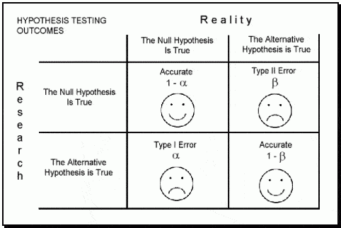 |
| Image taken from: https://datasciencedojo.com/ |
The probability of incurring in a type I error is indicated by α (or significance level) and usually takes a value of 5%; this means that we are happy to consider a scenario where we have 5% chances of rejecting the null hypothesis when it is actually true. If we are not happy with this, we can further decrease this probability by decreasing the value of α (for example to 1%). On the contrary the probability of incurring in a type II error is expressed by β, which usually takes a value of 20% (meaning a power of 80%). This means we are happy to work assuming that we have a 20% chance of accepting the null hypothesis when it is actually false.
If our experiment is not designed properly we cannot be sure whether we actually incurred in one of these two errors. In other words, if we run a bad experiment and we obtain a insignificant p-value it may be that we incurred in a type II error, meaning that in reality our treatment works but its effect cannot be detected by our experiment. However, it may also be that we obtained a significant p-value but we incurred in a type I error, and if we repeat the experiment we will find different results.
The only way we can be sure to run a good experiment is by running a power analysis. By definition power is the probability of obtaining statistical significance (not necessarily a small p-value, but at least a realistic outcome). Power analysis can be used before an experiment to test whether our design has good chances of succeeding (a priori) or after to test whether the results we obtained were realistic.
Update 17/11/2017
How many subjects to compute a robust mean?
This is a question that I get sometimes when talking with students that are planning descriptive experiments. How many subjects do I need for the mean value I compute to be robust?The answer is provided by Berkowitz here: www.columbia.edu/~mvp19/RMC/M6/M6.doc
The simplified formula to compute the minimum number of samples is:

where SD is the standard deviation and SE is the standard error. These values can be obtained from previous experiments, or from the literature.
Effect Size
A simple and effective definition of effect size is provided in the book "Power Analysis for Experimental Research" by Bausell & Li. They say:
"effect size is nothing more than a standardized measure of the size of the mean difference(s) among the study’s groups or of the strength of the relationship(s) among its variables".
Despite its simple definition the calculation of the effect size is not always straightforward and many indexes have been proposed over the years. Bausell & Li propose the following definition, in line with what proposed by Cohen in his "Statistical Power Analysis for the Behavioral Sciences":


This is the main definition but then every software or functions tend to use indexes correlated to this but not identical. We will see each way of calculating the effect size case by case.
One-Way ANOVA
Sample size
For simple models the power calculating can be performed with the package pwr:
library(pwr)
In the previous post (Linear Models) we worked on a dataset where we tested the impact on yield of 6 levels of nitrogen. Let's assume that we need to run a similar experiment and we would like to know how many samples we should collect (or how many plants we should use in the glass house) for each level of nitrogen. To calculate this we need to do a power analysis.
To compute the sample size required to reach good power we can run the following line of code:
Let's start describing the options from the end. We have the option power, to specify the power you require for your experiment. In general, this can be set to 0.8, as mentioned above. The significance level is alpha and usually we are happy to accept a significance of 5%. Another option is k, which is the number of groups in our experiment, in this case we have 6 groups.
Finally we have the option f, which is the effect size. As I mentioned above, there are many indexes to express the effect size and f is one of them.
According to Cohen, f can be expressed as:

where the numerator is the is the standard deviation of the effects that we want to test and the denominator is the common standard deviation. For two means, as in the equation we have seen above, f is simply equal to:

Clearly, before running the experiment we do not really know what the effect size would be. In some case we may have an idea, for example from previous experiments or a pilot study. However, most of the times we do not have a clue. In such cases we can use the classification suggested by Cohen, who considered the following values for f:
 The general rule is that if we do not know anything about our experiment we should use a medium effect size, so in this case 0.25. This was suggested in the book Bausell & Li and it is based on a review of 302 studies in the social and behavioral sciences. for this reason it may well be that the effect size of your experiment would be different. However, if you do not have any additional information this is the only thing the literature suggest.
The function above returns the following output:
In this example we would need 36 samples for each nitrogen level to achieve a power of 80% with a significance of 5%.
Let's start from d, which can be simply calculated using means and standard deviation of two groups, for example N0 (control) and N5:
This code simply computes the numerator (difference in means) and the denominator (pooled standard deviation) and then computes the Cohen's d, you just need to change the vectors for objects Control and Treatment1. The effect size results in 0.38.
Again Cohen provides some values for the d, so that we can determine how large is our effects, which are presented below:
 From this table we can see that our effect size is actually low, and not medium as we assumed for the a priori analysis. This is important because if we run the experiment with 36 samples per group we may end up with unrealistic results simply due to low power. For this reason it is my opinion that we should always be a bit more conservative and maybe include some additional replicates or blocks, just to account for potential unforeseen differences between our assumptions and reality.
The function to compute power is again pwr.anova.test, in which the effect size is expressed as f. We have two ways of doing that, the first is by using the d values we just calculated and halve it, so in this case f = 0.38/2 = 0.19. However, this will tell you the specific effects size for the relation between N0 and N5, and not for the full set of treatments.
NOTE:
At this link there is an Excel file that you can use to convert between indexes of effect size:
http://www.stat-help.com/spreadsheets/Converting%20effect%20sizes%202012-06-19.xls
Another way to get a fuller picture is by using the partial Eta Squared, which can be calculated using the sum of squares:

This will tell us the average effect size for all the treatments we applied, so not only for N5 compared to N0, but for all of them.
To compute the partial eta squared we first need to access the anova table, with the function anova:
From this table we can extract the sum of squares for the treatment (i.e. nf) and the sum of squares of the residuals and then solve the equation above:
As for the other indexes, eta squares also has its table of interpretation:
 The relation between f and eta squared is the following:

so to compute the f related to the full treatment we can simply do the following:
So now we have everything we need to calculate the power of our model:
To compute the power we need to run again the function pwr.anova.test, but this time without specifying the option power, but replacing it with the option n, which is the number of samples per group.
As you remember from the previous post this was an unbalanced design, so the number of samples per group is not constant. We could either use a vector as input for n, with all the samples per each group. In that case the function will return a power for each group. However, what I did here is putting the lowest number, so that we are sure to reach good power for the lowest sample size.
As you can see even with the small effect size we are still able to reach a power of 1, meaning 100%. This is because the sample size is more than adequate to catch even such a small effect. You could try to run again the sample size calculation to actually see what would be the minimum sample requirement for the observed effect size.
To compute the sample size required to reach good power we can run the following line of code:
pwr.anova.test(k=6, f=0.25, sig.level=0.05, power=0.8)
Let's start describing the options from the end. We have the option power, to specify the power you require for your experiment. In general, this can be set to 0.8, as mentioned above. The significance level is alpha and usually we are happy to accept a significance of 5%. Another option is k, which is the number of groups in our experiment, in this case we have 6 groups.
Finally we have the option f, which is the effect size. As I mentioned above, there are many indexes to express the effect size and f is one of them.
According to Cohen, f can be expressed as:

where the numerator is the is the standard deviation of the effects that we want to test and the denominator is the common standard deviation. For two means, as in the equation we have seen above, f is simply equal to:

Clearly, before running the experiment we do not really know what the effect size would be. In some case we may have an idea, for example from previous experiments or a pilot study. However, most of the times we do not have a clue. In such cases we can use the classification suggested by Cohen, who considered the following values for f:

The function above returns the following output:
 > pwr.anova.test(k=6, f=0.25, sig.level=0.05, power=0.8)
    Balanced one-way analysis of variance power calculation
        k = 6
        n = 35.14095
        f = 0.25
    sig.level = 0.05
      power = 0.8
 NOTE: n is number in each group
In this example we would need 36 samples for each nitrogen level to achieve a power of 80% with a significance of 5%.
Power Calculation
As I mentioned above, sometimes we have a dataset we collected assuming we could reach good power but we are not actually sure if that is the case. In those instances what we can do is the a posteriori power analysis, where we basically compute the power for a model we already fitted.
As you remember is the previous post about linear models, we fitted the following:
To compute the power we achieved here we first need to calculate the effect size. As discussed above we have several options: d, f and another index called partial eta squared. mod1 = aov(yield ~ nf, data=dat)
Let's start from d, which can be simply calculated using means and standard deviation of two groups, for example N0 (control) and N5:
 Control = dat[dat$nf=="N0","yield"]
 Treatment1 = dat[dat$nf=="N5","yield"]

 numerator = (mean(Treatment1)-mean(Control))
 denominator = sqrt((((length(Treatment1)-1)*sd(Treatment1)^2)+((length(Control)-1)*sd(Control)^2))/(length(Treatment1)+length(Control)-2))

 d = numerator/denominator
This code simply computes the numerator (difference in means) and the denominator (pooled standard deviation) and then computes the Cohen's d, you just need to change the vectors for objects Control and Treatment1. The effect size results in 0.38.
Again Cohen provides some values for the d, so that we can determine how large is our effects, which are presented below:

The function to compute power is again pwr.anova.test, in which the effect size is expressed as f. We have two ways of doing that, the first is by using the d values we just calculated and halve it, so in this case f = 0.38/2 = 0.19. However, this will tell you the specific effects size for the relation between N0 and N5, and not for the full set of treatments.
NOTE:
At this link there is an Excel file that you can use to convert between indexes of effect size:
http://www.stat-help.com/spreadsheets/Converting%20effect%20sizes%202012-06-19.xls
Another way to get a fuller picture is by using the partial Eta Squared, which can be calculated using the sum of squares:

This will tell us the average effect size for all the treatments we applied, so not only for N5 compared to N0, but for all of them.
To compute the partial eta squared we first need to access the anova table, with the function anova:
 > anova(mod1)
 Analysis of Variance Table
 Response: yield
       Df Sum Sq Mean Sq F value  Pr(>F)
 nf      5  23987 4797.4 12.396 6.075e-12 ***
 Residuals 3437 1330110  387.0
 ---
 Signif. codes: 0 ‘***’ 0.001 ‘**’ 0.01 ‘*’ 0.05 ‘.’ 0.1 ‘ ’ 1
From this table we can extract the sum of squares for the treatment (i.e. nf) and the sum of squares of the residuals and then solve the equation above:
 > EtaSQ = 23987/(23987+1330110)
 > print(EtaSQ)
 [1] 0.01771439
As for the other indexes, eta squares also has its table of interpretation:


so to compute the f related to the full treatment we can simply do the following:
 > f = sqrt(EtaSQ / (1-EtaSQ))
 > print(f)
 [1] 0.1342902
So now we have everything we need to calculate the power of our model:
 > pwr.anova.test(k=6, n=571, f=f, sig.level=0.05)
    Balanced one-way analysis of variance power calculation
        k = 6
        n = 571
        f = 0.1342902
    sig.level = 0.05
      power = 1
 NOTE: n is number in each group
To compute the power we need to run again the function pwr.anova.test, but this time without specifying the option power, but replacing it with the option n, which is the number of samples per group.
As you remember from the previous post this was an unbalanced design, so the number of samples per group is not constant. We could either use a vector as input for n, with all the samples per each group. In that case the function will return a power for each group. However, what I did here is putting the lowest number, so that we are sure to reach good power for the lowest sample size.
As you can see even with the small effect size we are still able to reach a power of 1, meaning 100%. This is because the sample size is more than adequate to catch even such a small effect. You could try to run again the sample size calculation to actually see what would be the minimum sample requirement for the observed effect size.
Linear Model
The method we have seen above is only valid for one-way ANOVAs. For more complex model, which may simply be ANOVA with two treatments we should use the function specific for linear models.
Sample Size
To calculate the sample size for this analysis we can refer once again to the package pwr, but now use the function pwr.f2.test.Using this function is slightly more complex because here we start reasoning in terms of degrees of freedom for the F ratio, which can be obtained using the following equation:
 |
| From: https://cnx.org/contents/crKQFJtQ@14/F-Distribution-and-One-Way-ANO |
These two terms have the following equations (again from: https://cnx.org/contents/crKQFJtQ@14/F-Distribution-and-One-Way-ANO) :


The degrees of freedom we need to consider are the denominators of the last two equations. For an a priori power analysis we need to input the option u, with the degrees of freedom of the numerator of the F ratio, thus MS between. As you can see this can be computed as k-1, for a one-way ANOVA.
For more complex model we need to calculate the degrees of freedom ourselves. This is not difficult because we can generate dummy datasets in R with the specific treatment structure we require, so that R will compute the degrees of freedom for us.
We can generate dummy dataset very easily with the function expand.grid:
 > data = expand.grid(rep=1:3, FC1=c("A","B","C"), FC2=c("TR1","TR2"))
 > data
   rep FC1 FC2
 1  1  A TR1
 2  2  A TR1
 3  3  A TR1
 4  1  B TR1
 5  2  B TR1
 6  3  B TR1
 7  1  C TR1
 8  2  C TR1
 9  3  C TR1
 10  1  A TR2
 11  2  A TR2
 12  3  A TR2
 13  1  B TR2
 14  2  B TR2
 15  3  B TR2
 16  1  C TR2
 17  2  C TR2
 18  3  C TR2
Working with expand.grid is very simple. We just need to specify the level for each treatment and the number of replicates (or blocks) and the function will generate a dataset with every combination.
Now we just need to add the dependent variable, which we can generate randomly from a normal distribution:
data$Y = rnorm(nrow(data))
Now our dataset is ready so we can fit a linear model to it and generate the ANOVA table:
 > mod.pilot = lm(Y ~ FC1*FC2, data=data)
 > anova(mod.pilot)
 Analysis of Variance Table
 Response: Y
      Df Sum Sq Mean Sq F value Pr(>F)
 FC1    2 0.8627 0.4314 0.3586 0.7059
 FC2    1 3.3515 3.3515 2.7859 0.1210
 FC1:FC2  2 1.8915 0.9458 0.7862 0.4777
 Residuals 12 14.4359 1.2030
Since this is a dummy dataset all the sum of squares and the other values are meaningless. We are only interested in looking at the degrees of freedom.
To calculate the sample size for this analysis we can refer once again to the package pwr, but now use the function pwr.f2.test, as follows:
pwr.f2.test(u = 2, f2 = 0.25, sig.level = 0.05, power=0.8)
The first option in the function is u, which represents the degrees of freedom of the numerator of the F ratio. This is related to the degrees of freedom of the component we want to focus on. As you probably noticed from the model, we are trying to see if there is an interaction between two treatments. From the ANOVA table above we can see that the degrees of freedom of the interaction are equal to 2, so that it what we include as u.
Other options are again power and significance level, which we already discussed. Moreover, in this function the effect size is f2, which is again different from the f we've seen before. F2 again has its own table:

The function returns the following table:
 > pwr.f2.test(u = 2, f2 = 0.25, sig.level = 0.05, power=0.8)
    Multiple regression power calculation
        u = 2
        v = 38.68562
        f2 = 0.25
    sig.level = 0.05
      power = 0.8
As you can see what the function is actually providing us is the value of the degrees of freedom for the denominator of the F test (with v), which results in 38.68, so 39 since we always round it by excess.
If we look to the equation to compute MS withing we can see that the degrees of freedom is given by n-k, meaning that to transform the degrees of freedom into a sample size we need to add what we calculated before for the option u. The sample size is then equal to n = v + u + 1, so in this case the sample size is equal 39 + 2 + 1 = 42
This is not the number of samples per group but it is the total number of samples.
Another way of looking at the problem would be to compute the total power of our model, and not just how much power we have to discriminate between levels of one of the treatments (as we saw above). To do so we can still use the function pwr.f2.test, but with some differences. The first is that we need to compute u using all elements in the model, so basically sum the decrees of freedom of the ANOVA table, or sum all the coefficients in the model minus the intercept:
u = length(coef(mod3))-1
Another difference is in how we compute the effects size f2. Before we used its relation with partial eta square, now we can use its relation with the R2 of the model:

With these additional element we can compute the power of the model.
Power Calculation
Now we look at estimating the power for a model we've already fitted, which can be done with the same function.
mod3 = lm(yield ~ nf + bv, data=dat)
Once again we first need to calculate the observed effect size as the eta squared, using again the sum of squares:
 > Anova(mod3, type="III")
 Anova Table (Type III tests)
 Response: yield
       Sum Sq  Df F value  Pr(>F)
 (Intercept) 747872  1 2877.809 < 2.2e-16 ***
 nf      24111  5  18.555 < 2.2e-16 ***
 bv     437177  1 1682.256 < 2.2e-16 ***
 Residuals  892933 3436
 ---
 Signif. codes: 0 ‘***’ 0.001 ‘**’ 0.01 ‘*’ 0.05 ‘.’ 0.1 ‘ ’ 1
In this example, I used the function Anova (with option type="III") in the package car just to remind you that if you have an unbalanced design, like in this case, you should use the type III sum of squares.
From this table we can obtain the sum of squares we need to compute the eta squared, for example for nf we will use the following code:
 > EtaSQ = 24111/(24111+892933)
 > EtaSQ
 [1] 0.02629209
Then we need to transform this into f2 (of f squared), which is what the pwr.f2.test function uses:
 > f2 = EtaSQ / (1-EtaSQ)
 > f2
 [1] 0.02700203
The only thing we need to do now is calculating the value of v, i.e. the denominator degrees of freedom. This is equal to the n (number of samples) - u - 1, but a quick way of obtaining this number is looking at the anova table above and take the degrees of freedom of the residuals, i.e. 3436.
Now we have everything we need to obtain the observed power:
 > pwr.f2.test(u = 5, v = 3436, f2 = f2, sig.level = 0.05)
    Multiple regression power calculation
        u = 5
        v = 3436
        f2 = 0.02700203
    sig.level = 0.05
      power = 1
which again returns a very high power, since we have a lot of samples.
Generalized Linear Models
For GLM we need to install the package lmsupport:
 #install.packages("lmSupport")
 library(lmSupport)
Sample Size
For calculating the sample size for GLM we can use the same procedure we used for linear models.Power Calculation
For this example we are going to use one of the model we discussed in the post about GLM, using the dataset beall.webworms (n = 1300):
 dat = beall.webworms
 pois.mod2 = glm(y ~ block + spray*lead, data=dat, family=c("poisson"))
Once again we would need to compute effect size and degrees of freedom. As before, we can use the function anova to generate the data we need:
 > anova(pois.mod2)
 Analysis of Deviance Table
 Model: poisson, link: log
 Response: y
 Terms added sequentially (first to last)
       Df Deviance Resid. Df Resid. Dev
 NULL            1299   1955.9
 block   12 122.040   1287   1833.8
 spray    1 188.707   1286   1645.2
 lead    1  42.294   1285   1602.8
 spray:lead 1  4.452   1284   1598.4
Let's say we are interested in looking at the interaction between spray and lead, its degrees of freedom are 1, so this is our u. On its side we also have the residuals degrees of freedom, so v is 1284.
The other thing we need is the effect size, which we can compute with the function modelEffectSizes from the package lmSupport:
 > modelEffectSizes(pois.mod2)
 glm(formula = y ~ block + spray * lead, family = c("poisson"),
   data = dat)
 Coefficients
       SSR df pEta-sqr dR-sqr
 block 122.0402 12  0.0709   NA
 spray 142.3487 1  0.0818 0.0849
 lead  43.7211 1  0.0266 0.0261
 Sum of squared errors (SSE): 1598.4
 Sum of squared total (SST): 1675.9
This function calculates the partial eta squares, and it works also for lm models. As you can see it does not provide the eta squared for the interaction, but just to be on the safe side we can use the lowest value (0.03) from the values provided for spray and lead.
Now that we have the observed eta squared we can use the function modelPower:
> modelPower(u=1, v=1284, alpha=0.05, peta2=0.03)
Results from Power Analysis

pEta2 = 0.030
u =     1
v =     1284.0
alpha = 0.050
power = 1.000
This function can take the option f2, as we've seen before for the package pwr. However, since computing the partial eta square is generally easier, we can use the option peta2 and use directly this index.
Once again our power is very high.
Note 12/12/2017
Please note that the line above only works with the older version of the package lmSupport (version 2.9.8). The new version features a different syntax.You can download the old version from here: https://cran.r-project.org/src/contrib/Archive/lmSupport/lmSupport_2.9.8.tar.gz
Linear Mixed Effects Models
For power analysis with mixed effects models we would need to install the following packages:
 #install.packages("simr")
 library(simr)
In this example we will be working with models fitted with the package lme4, but what is discussed here should work also with models fitted with nlme.
Sample Size
A priori power analysis for mixed effect model is not easy. There are packages that should provide functions to do that (e.g. simstudy and longpower), but they are probably more related to the medical sciences and I found them difficult to use. For this reason I decided that probably the easiest way to test the power of an experiment for which we need to use a mixed-effect model (e.g. involving clustering or repeated measures) would be to use a dummy dataset again and simulation. However, please be advised that I am not 100% sure of the validity of this procedure.
To create the dummy dataset we can use the same procedure we employed above, with expand.grid:
 data = expand.grid(subject=1:5, treatment=c("Tr1", "Tr2", "Tr3"))
 data$Y = numeric(nrow(data))
In this case we are simulating a simple experiment with 5 subjects, 3 treatments and a within subject design, like a crossover I suppose.
As you can see the Y has not been drawn from a normal distribution, this is because for the time being it is just a list of zeroes. We need to create data for each treatment as follows:
As you can see the Y has not been drawn from a normal distribution, this is because for the time being it is just a list of zeroes. We need to create data for each treatment as follows:
 data[data$treatment=="Tr1","Y"] = rnorm(nrow(data[data$treatment=="Tr1",]), mean=20, sd=1)
 data[data$treatment=="Tr2","Y"] = rnorm(nrow(data[data$treatment=="Tr2",]), mean=20.5, sd=1)
 data[data$treatment=="Tr3","Y"] = rnorm(nrow(data[data$treatment=="Tr3",]), mean=21, sd=1)
In these lines I created three samples, from normal distributions, which means differ by half their standard deviation. This (when SD = 1) provides an effect size (d) of 0.5, so medium.
Now we can create the model:
Now we can create the model:
 mod1 = lmer(Y ~ treatment + (1|subject), data=data)
 summary(mod1)
and then test its power with the function powerSim from the package simr. This function runs 1000 simulation and provide a measure for the power of the experiment:
 > powerSim(mod1, alpha=0.05)
 Power for predictor 'treatment', (95% confidence interval):
    25.90% (23.21, 28.73)
 Test: Likelihood ratio
 Based on 1000 simulations, (84 warnings, 0 errors)
 alpha = 0.05, nrow = 15
 Time elapsed: 0 h 3 m 2 s
 nb: result might be an observed power calculation
 Warning message:
 In observedPowerWarning(sim) :
  This appears to be an "observed power" calculation
Let's now look at repeated measures. In this case we do not only have the effect size to account for in the data, but also the correlation between in time between measures.
 library(mvtnorm)

 sigma <- matrix(c(1, 0.5, 0.5, 0.5,
          0.5, 1, 0.5, 0.5,
          0.5, 0.5, 1, 0.5,
                0.5, 0.5, 0.5 ,1 ), ncol=4, byrow=T)


 data = expand.grid(subject=1:4, treatment=c("Tr1", "Tr2", "Tr3"), time=c("t1","t2","t3","t4"))
 data$Y = numeric(nrow(data))

 T1 = rmvnorm(4, mean=rep(20, 4), sigma=sigma)
 T2 = rmvnorm(4, mean=rep(20.5, 4), sigma=sigma)
 T3 = rmvnorm(4, mean=rep(21, 4), sigma=sigma)

 data[data$subject==1&data$treatment=="Tr1","Y"] = T1[,1]
 data[data$subject==2&data$treatment=="Tr1","Y"] = T1[,2]
 data[data$subject==3&data$treatment=="Tr1","Y"] = T1[,3]
 data[data$subject==4&data$treatment=="Tr1","Y"] = T1[,4]

 data[data$subject==1&data$treatment=="Tr2","Y"] = T2[,1]
 data[data$subject==2&data$treatment=="Tr2","Y"] = T2[,2]
 data[data$subject==3&data$treatment=="Tr2","Y"] = T2[,3]
 data[data$subject==4&data$treatment=="Tr2","Y"] = T2[,4]

 data[data$subject==1&data$treatment=="Tr3","Y"] = T3[,1]
 data[data$subject==2&data$treatment=="Tr3","Y"] = T3[,2]
 data[data$subject==3&data$treatment=="Tr3","Y"] = T3[,3]
 data[data$subject==4&data$treatment=="Tr3","Y"] = T3[,4]


 modRM = lmer(Y ~ treatment + (time|subject), data=data)
 summary(modRM)

 powerSim(modRM, alpha=0.05)
In this case we need to use the function rmvnorm to draw, from a normal distribution, samples with a certain correlation. For this example I followed the approach suggested by William Huber here: https://stats.stackexchange.com/questions/24257/how-to-simulate-multivariate-outcomes-in-r/24271#24271
Basically, if we assume a correlation equal to 0.5 between time samples (which is what the software G*Power does for repeated measures), we first need to create a symmetrical matrix in sigma. This will allow rmvnorm to produce values from distributions with standard deviation equal to 1 and 0.5 correlation.
A more elegant approach is the one suggested by Ben Amsel on his blog: https://cognitivedatascientist.com/2015/12/14/power-simulation-in-r-the-repeated-measures-anova-5/
 sigma = 1 # population standard deviation
 rho = 0.5 #Correlation between repeated measurs
 # create k x k matrix populated with sigma
 sigma.mat <- rep(sigma, 4)
 S <- matrix(sigma.mat, ncol=length(sigma.mat), nrow=length(sigma.mat))
 # compute covariance between measures
 Sigma <- t(S) * S * rho
 # put the variances on the diagonal
 diag(Sigma) <- sigma^2
The result is the same but at least here you can specify different values for SD and correlation.
The other elementS the function needs are mean values, for which I used the same as before. This should guarantee a difference of around half a standard deviation between treatments.
The remaining of the procedure is the same we used before with no changes.
As I said before, I am not sure if this is the correct way of computing power for linear mixed effects models. It may be completely or partially wrong, and if you know how to do this or you have comments please do not hesitate to write them below.
Power Analysis
As we have seen with the a priori analysis, computing the power of mixed effects models is actually very easy with the function powerSim.References
PWR package Vignette: https://cran.r-project.org/web/packages/pwr/vignettes/pwr-vignette.htmlWilliam E. Berndtson (1991). "A simple, rapid and reliable method for selecting or assessing the number of replicates for animal experiments"
http://scholars.unh.edu/cgi/viewcontent.cgi?article=1312&context=nhaes
NOTE:
This paper is what some of my colleagues, who deal particularly with animal experiments, use to calculate how many subjects to use for their experiments. The method presented here is base on the coefficient of variation (CV%), which is something that also in agriculture is often used to estimate the number of replicates needed.
Berkowitz J. "Sample Size Estimation" - http://www.columbia.edu/~mvp19/RMC/M6/M6.doc
This document gives you some rule of thumb to determine the sample size for a number of experiments.
Update 26/07/2017
For computing effect size automatically you also have the option to use the package sjstats. This has function to compute eta-squared, partial eta-squared and others, but it also has an option to print a comprehensive ANOVA table with everything you get from a normal call to anova plus the effects sizes.
You can find some example on this blog post from the author of the package Daniel Lüdecke here:
Final Note about the use of CV%
AS I mentioned above, CV% and the percentage of difference between means is one of the indexes used to estimate the number of replicates needed to run experiments. For this reason I decided to create some code to test whether power analysis and the method based on CV% provide similar results.
Below is the function I created for this:
 d.ES = function(n, M, SD, DV){
 M1=M
 M2=M+(SD/DV)
 PC.DIFF = (abs(M1-M2)/((M1+M2)/2))*100
 numerator = (mean(M2)-mean(M1))
 denominator = sqrt((((n-1)*SD^2)+((n-1)*SD^2))/(n+n-2))
 ES=numerator/denominator
 samp = sapply(ES, function(x){pwr.anova.test(k=2, f=x/2, sig.level=0.05, power=0.8)$n})
 CV1=SD/M1
 return(list(EffectSize=ES, PercentageDifference=PC.DIFF, CV.Control=CV1*100, n.samples=samp))
 }
This function takes 4 arguments: number of samples (n), mean of control (M), standard deviation (here we assume the standard deviation to be identical between groups), and DV, which indicates the number of times to divide the standard deviation to compute the mean of the treatment. If DV is equal to 2 then the mean of the treatment will be half the mean of control.
The equation for the percentage of difference was taken from: https://www.calculatorsoup.com/calculators/algebra/percent-difference-calculator.php
Now we can use this function to estimate Effect Size, percentage of differences in means, CV% and number of samples from power analysis (assuming an ANOVA with 2 groups).
The first example looks at changing the standard deviation, and keeping everything else constant:
 > d.ES(n=10, M=20, SD=seq(1, 15, by=1), DV=8)
 $EffectSize
  [1] 1.00000000 0.50000000 0.33333333 0.25000000 0.20000000 0.16666667
  [7] 0.14285714 0.12500000 0.11111111 0.10000000 0.09090909 0.08333333
 [13] 0.07692308 0.07142857 0.06666667
 $PercentageDifference
  [1] 0.623053 1.242236 1.857585 2.469136 3.076923 3.680982 4.281346 4.878049
  [9] 5.471125 6.060606 6.646526 7.228916 7.807808 8.383234 8.955224
 $CV.Control
  [1] 5 10 15 20 25 30 35 40 45 50 55 60 65 70 75
 $n.samples
  [1]  10.54166  39.15340  86.88807 153.72338 239.65639 344.68632
  [7] 468.81295 612.03614 774.35589 955.77211 1156.28483 1375.89403
 [13] 1614.59972 1872.40183 2149.30043
If you look at the tables presented in the paper by Berndtson you will see that the results are similar in terms of number of samples.
Larger differences are seen when we look at changes in mean, while everything else stays constant:
 > d.ES(n=10, M=seq(1,25,1), SD=5, DV=8)
 $EffectSize
 [1] 0.125
 $PercentageDifference
  [1] 47.619048 27.027027 18.867925 14.492754 11.764706 9.900990 8.547009
  [8] 7.518797 6.711409 6.060606 5.524862 5.076142 4.694836 4.366812
 [15] 4.081633 3.831418 3.610108 3.412969 3.236246 3.076923 2.932551
 [22] 2.801120 2.680965 2.570694 2.469136
 $CV.Control
  [1] 500.00000 250.00000 166.66667 125.00000 100.00000 83.33333 71.42857
  [8] 62.50000 55.55556 50.00000 45.45455 41.66667 38.46154 35.71429
 [15] 33.33333 31.25000 29.41176 27.77778 26.31579 25.00000 23.80952
 [22] 22.72727 21.73913 20.83333 20.00000
 $n.samples
 [1] 1005.615
In this case the mean of the treatment is again 1/8 of the mean of the control, and the standard deviation is fixed at 5. Since the difference in means is the same, and the standard deviation is constant, the effect size also stays constant at 0.125, so very small.
However, both percentage of difference and CV% change quite a bit and therefore the estimates from Berndtson could differ.


