Preface
I am writing this post more for reminding to myself some theoretical background and the steps needed to perform spatio-temporal kriging in gstat.
This month I had some free time to spend on small projects not specifically related to my primary occupation. I decided to spend some time trying to learn this technique since it may become useful in the future. However, I have never used it before so I had to first try to understand its basics both in terms of theoretical background and programming.
Since I have used several resources to get a handle on it, I decided to share my experience and thoughts on this blog post because they may become useful for other people trying the same method. However, this post cannot be considered a full review of spatio-temporal kriging and its theoretical basis. I just mentioned some important details to guide myself and the reader through the comprehension of the topic, but these are clearly not exhaustive. At the end of the post I included some references to additional material you may want to browse for more details.
Introduction
This is the first time I considered spatio-temporal interpolation. Even though many datasets are indexed in both space and time, in the majority of cases time is not really taken into account for the interpolation. As an example we can consider temperature observations measured hourly from various stations in a determined study area. There are several different things we can do with such a dataset. We could for instance create a series of maps with the average daily or monthly temperatures. Time is clearly considered in these studies, but not explicitly during the interpolation phase. If we want to compute daily averages we first perform the averaging and then kriging. However, the temporal interactions are not considered in the kriging model.
An example of this type of analysis is provided by (Gräler, 2012) in the following image, which depicts monthly averages for some environmental parameter in Germany:
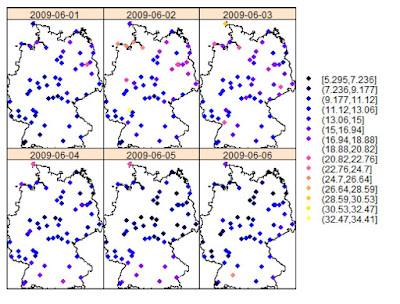
There are cases and datasets in which performing 2D kriging on “temporal slices” may be appropriate. However, there are other instances where this is not possible and therefore the only solution is take time into account during kriging. For doing so two possible solutions are suggested in literature: using time as a third dimension, or fit a covariance model with both spatial and temporal components (Gräler et al., 2013).
Time as the third dimension
The idea behind this technique is extremely easy to grasp. To better understand it we can simply take a look at the equation to calculate the sample semivariogram, from Sherman (2011):

Under Matheron’s Intrinsic Hypothesis (Oliver et al., 1989) we can assume that the variance between two points, si and sj, depends only on their separation, which we indicate with the vector h in Eq.1. If we imagine a 2D example (i.e. purely spatial), the vector h is simply the one that connects two points, i and j, with a line, and its value can be calculated with the Euclidean distance:

If we consider a third dimension, which can be depth, elevation or time; it is easy to imagine Eq.2 be adapted to accommodate an additional dimension.
The only problem with this method is that in order for it to work properly the temporal dimension needs to have a range similar to the spatial dimension. For this reason time needs to be scaled to align it with the spatial dimension. In Gräler et al. (2013) they suggest several ways to optimize the scaling and achieve meaningful results. Please refer to this article for more information.
Spatio-Temporal Variogram
The second way of taking time into account is to adapt the covariance function to the time component. In this case for each point si there will be a time ti associated with it, and to calculate the variance between this point and another we would need to calculate their spatial separation h and their temporal separation u. Thus, the spatio-temporal variogram can be computed as follows, from Sherman (2011):

With this equation we can compute a variogram taking into account every pair of points separated by distance h and time u.
Spatio-Temporal Kriging in R
In R we can perform spatio-temporal kriging directly from gstat with a set of functions very similar to what we are used to in standard 2D kriging. The package spacetime provides ways of creating objects where the time component is taken into account, and gstat uses these formats for its space-time analysis. Here I will present an example of spatio-temporal kriging using sensors’ data.
Data
In 2011, as part of the OpenSense project, several wireless sensors to measure air pollution (O3, NO2, NO, SO2, VOC, and fine particles) were installed on top of trams in the city of Zurich. The project now is in its second phase and more information about it can be found here: http://www.opensense.ethz.ch/trac/wiki/WikiStart
In this page some examples data about Ozone and Ultrafine particles are also distributed in csv format. These data have the following characteristics: time is in UNIX format, while position is in degrees (WGS 84). I will use these data to test spatio-temporal kriging in R.
Packages
To complete this exercise we need to load several packages. First of all sp, for handling spatial objects, and gstat, which has all the function to actually perform spatio-temporal kriging. Then spacetime, which we need to create the spatio-temporal object. These are the three crucial packages. However, I also loaded some others that I used to complete smaller tasks. I loaded the raster package, because I use the functions
coordinates and projection to create spatial data. There is no need of loading it, since the same functions are available under different names in sp. However, I prefer these two because they are easier to remember. The last packages are rgdal and rgeos, for performing various operations on geodata.
The script therefore starts like:
Data Preparation
There are a couple of issues to solve before we can dive into kriging. The first is that we need to do is translating the time from UNIX to
POSIXlt or POSIXct, which are standard ways of representing time in R. This very first thing we have to do is of course setting the working directory and loading the csv file:setwd("...") data <- read.table("ozon_tram1_14102011_14012012.csv", sep=",", header=T)
Now we need to address the UNIX time. So what is UNIX time anyway?
It is a way of tracking time as the number of seconds between a particular time and the UNIX epoch, which is January the 1st 1970 GMT. Basically, I am writing the first draft of this post on August the 18th at 16:01:00 CET. If I count the number of seconds from the UNIX epoch to this exact moment (there is an app for that!!) I find the UNIX time, which is equal to: 1439910060
Now let's take a look at one entry in the column “generation_time” of our dataset:
As you may notice here the UNIX time is represented by 13 digits, while in the example above we just had 10. The UNIX time here represents also the milliseconds, which is something we cannot represent in R (as far as I know). So we cannot just convert each numerical value into
POSIXlt, but we first need to extract only the first 10 digits, and then convert it. This can be done in one line of code but with multiple functions:data$TIME <- as.POSIXlt(as.numeric(substr(paste(data$generation_time), 1, 10)), origin="1970-01-01")
We first need to transform the UNIX time from numerical to character format, using the function
paste(data$generation_time). This creates the character string shown above, which we can then subset using the function substr. This function is used to subtract characters from a string and takes three arguments: a string, a starting character and a stopping character. In this case we want to basically delete the last 3 numbers from our string, so we set the start on the first number (start=1), and the stop at 10 (stop=10). Then we need to change the numerical string back to a numerical format, using the function as.numeric. Now we just need one last function to tell R that this particular number is a Date/Time object. We can do this using the function as.POSIXlt, which takes the actual number we just created plus an origin. Since we are using UNIX time, we need to set the starting point at "1970-01-01". We can test this function of the first element of the vector data$generation_time to test its output: > as.POSIXlt(as.numeric(substr(paste(data$generation_time[1]), start=1, stop=10)), origin="1970-01-01") [1] "2011-10-14 11:14:46 CEST"
Now the
data.frame data has a new column named TIME where the Date/Time information are stored.
Another issue with this dataset is in the formats of latitude and longitude. In the csv files these are represented in the format below:
Basically geographical coordinates are represented in degrees and minutes, but without any space. For example, for this point the longitude is 8°32.88’, while the latitude is 47°24.22’. For obtaining coordinates with a more manageable format we would again need to use strings.
data$LAT <- as.numeric(substr(paste(data$latitude),1,2))+(as.numeric(substr(paste(data$latitude),3,10))/60)

data$LON <- as.numeric(substr(paste(data$longitude),1,1))+(as.numeric(substr(paste(data$longitude),2,10))/60)
We use again a combination of
paste and substr to extract only the numbers we need. For converting this format into degrees, we need to sum the degrees with the minutes divided by 60. So in the first part of the equation we just need to extract the first two digits of the numerical string and transform them back to numerical format. In the second part we need to extract the remaining of the strings, transform them into numbers and then divided them by 60.This operation creates some NAs in the dataset, for which you will get a warning message. We do not have to worry about it as we can just exclude them with the following line: Subset
The ozone dataset by OpenSense provides ozone readings every minute or so, from October the 14th 2011 at around 11 a.m., up until January the 14th 2012 at around 2 p.m.
The size of this dataset is 200183 rows, which makes it kind of big for perform kriging without a very powerful machine. For this reason before we can proceed with this example we have to subset our data to make them more manageable. To do so we can use the standard subsetting method for
data.frame objects using Date/Time:> sub <- data[data$TIME>=as.POSIXct('2011-12-12 00:00 CET')&data$TIME<=as.POSIXct('2011-12-14 23:00 CET'),] > nrow(sub) [1] 6734
Here I created an object named sub, in which I used only the readings from midnight on December the 12th to 11 p.m. on the 14th. This creates a subset of 6734 observations, for which I was able to perform the whole experiment using around 11 Gb of RAM.
After this step we need to transform the object sub into a spatial object, and then I changed its projection into UTM so that the variogram will be calculated on metres and not degrees. These are the steps required to achieve all this:
Now we have the object ozone.UTM, which is a
SpatialPointsDataFrame with coordinates in metres.
Spacetime Package
Gstat is able to perform spatio-temporal kriging exploiting the functionalities of the package spacetime, which was developed by the same team as gstat. In spacetime we have two ways to represent spatio-temporal data:
STFDF and STIDF formats. The first represents objects with a complete space time grid. In other words in this category are included objects such as the grid of weather stations presented in Fig.1. The spatio-temporal object is created using the n locations of the weather stations and the m time intervals of their observations. The spatio-temporal grid is of size nxm. STIDF objects are the one we are going to use for this example. These are unstructured spatio-temporal objects, where both space and time change dynamically. For example, in this case we have data collected on top of trams moving around the city of Zurich. This means that the location of the sensors is not consistent throughout the sampling window.
Creating
STIDF objects is fairly simple, we just need to disassemble the data.frame we have into a spatial, temporal and data components, and then merge them together to create the STIDF object.
The first thing to do is create the
SpatialPoints object, with the locations of the sensors at any given time:
ozoneSP <- SpatialPoints(ozone.UTM@coords,CRS("+init=epsg:3395"))
This is simple to do with the function
At this point we need to perform a very important operation for kriging, which is check whether we have some duplicated points. It may happen sometime that there are points with identical coordinates. Kriging cannot handle this and returns an error, generally in the form of a “singular matrix”. Most of the time in which this happens the problem is related to duplicated locations. So we now have to check if we have duplicates here, using the function
SpatialPoints in the package sp. This function takes two arguments, the first is a matrix or a data.frame with the coordinates of each point. In this case I used the coordinates of the SpatialPointsDataFrame we created before, which are provided in a matrix format. Then I set the projection in UTM.At this point we need to perform a very important operation for kriging, which is check whether we have some duplicated points. It may happen sometime that there are points with identical coordinates. Kriging cannot handle this and returns an error, generally in the form of a “singular matrix”. Most of the time in which this happens the problem is related to duplicated locations. So we now have to check if we have duplicates here, using the function
zerodist:dupl <- zerodist(ozoneSP)
It turns out that we have a couple of duplicates, which we need to remove. We can do that directly in the two lines of code we would need to create the data and temporal component for the
STIDF object:ozoneDF <- data.frame(PPB=ozone.UTM$ozone_ppb[-dupl[,2]])
In this line I created a
data.frame with only one column, named PPB, with the ozone observations in part per billion. As you can see I removed the duplicated points by excluding the rows from the object ozone.UTM with the indexes included in one of the columns of the object dupl. We can use the same trick while creating the temporal part:ozoneTM <- as.POSIXct(ozone.UTM$TIME[-dupl[,2]],tz="CET")
Now all we need to do is combine the objects ozoneSP, ozoneDF and ozoneTM into a
STIDF:timeDF <- STIDF(ozoneSP,ozoneTM,data=ozoneDF)
This is the file we are going to use to compute the variogram and perform the spatio-temporal interpolation. We can check the raw data contained in the
STIDF object by using the spatio-temporal version of the function spplot, which is stplot:stplot(timeDF)

Variogram
The actual computation of the variogram at this point is pretty simple, we just need to use the appropriate function:
variogramST. Its use is similar to the standard function for spatial kriging, even though there are some settings for the temporal component that need to be included.
As you can see here the first part of the call to the function
I must warn you that this operation takes quite a long time, so please be aware of that. I personally ran it overnight.
variogramST is identical to a normal call to the function variogram; we first have the formula and then the data source. However, then we have to specify the time units (tunits) or the time lags (tlags). I found the documentation around this point a bit confusing to be honest. I tested various combinations of parameters and the line of code I presented is the only one that gives me what appear to be good results. I presume that what I am telling to the function is to aggregate the data to the hours, but I am not completely sure. I hope some of the readers can shed some light on this!!I must warn you that this operation takes quite a long time, so please be aware of that. I personally ran it overnight.
Plotting the Variogram
Basically the spatio-temporal version of the variogram includes different temporal lags. Thus what we end up with is not a single variogram but a series, which we can plot using the following line:
which return the following image:

Among all the possible types of visualizations for spatio-temporal variogram, this for me is the easiest to understand, probably because I am used to see variogram models. However, there are also other ways available to visualize it, such as the variogram map:

And the 3D wireframe:

Variogram Modelling
As in a normal 2D kriging experiment, at this point we need to fit a model to our variogram. For doing so we will use the function
Below I present the code I used to fit all the models. For the automatic fitting I used most of the settings suggested in the following demo:
vgmST and fit.StVariogram, which are the spatio-temporal matches for vgm and fit.variogram.Below I present the code I used to fit all the models. For the automatic fitting I used most of the settings suggested in the following demo:
demo(stkrige)
Regarding the variogram models, in gstat we have 5 options: separable, product sum, metric, sum metric, and simple sum metric. You can find more information to fit these model, including all the equations presented below, in (Gräler et al., 2015), which is available in pdf (I put the link in the "More Information" section).
Separable
This covariance model assumes separability between the spatial and the temporal component, meaning that the covariance function is given by:

According to (Sherman, 2011): “While this model is relatively parsimonious and is nicely interpretable, there are many physical phenomena which do not satisfy the separability”. Many environmental processes for example do not satisfy the assumption of separability. This means that this model needs to be used carefully.
The first thing to set are the upper and lower limits for all the variogram parameters, which are used during the automatic fitting:
The first thing to set are the upper and lower limits for all the variogram parameters, which are used during the automatic fitting:
# lower and upper bounds
pars.l <- c(sill.s = 0, range.s = 10, nugget.s = 0,sill.t = 0, range.t = 1, nugget.t = 0,sill.st = 0, range.st = 10, nugget.st = 0, anis = 0)
pars.u <- c(sill.s = 200, range.s = 1000, nugget.s = 100,sill.t = 200, range.t = 60, nugget.t = 100,sill.st = 200, range.st = 1000, nugget.st = 100,anis = 700)
To create a separable variogram model we need to provide a model for the spatial component, one for the temporal component, plus the overall sill:
This line creates a basic variogram model, and we can check how it fits our data using the following line:

One thing you may notice is that the variogram parameters do not seem to have anything in common with the image shown above. I mean, in order to create this variogram model I had to set the sill of the spatial component at -60, which is total nonsense. However, I decided to try to fit this model by-eye as best as I could just to show you how to perform this type of fitting and calculate its error; but in this case it cannot be taken seriously. I found that for the automatic fit the parameters selected for
We can check how this model fits our data by using the function
vgmST do not make much of a difference, so probably you do not have to worry too much about the parameters you select in vgmST.We can check how this model fits our data by using the function
fit.StVariogram with the option fit.method=0, which keeps this model but calculates its Mean Absolute Error (MSE), compared to the actual data:
This is basically the error of the eye fit. However, we can also use the same function to automatically fit the separable model to our data (here I used the settings suggested in the demo):
As you can see the error increases. This probably demonstrates that this model is not suitable for our data, even though with some magic we can create a pattern that is similar to what we see in the observations. In fact, if we check the fit by plotting the model it is clear that this variogram cannot properly describe our data:

To check the parameters of the model we can use the function
extractPar:> extractPar(separable_Vgm) range.s nugget.s range.t nugget.t sill 199.999323 10.000000 99.999714 1.119817 17.236256
Product Sum
A more flexible variogram model for spatio-temporal data is the product sum, which do not assume separability. The equation of the covariance model is given by:

with k > 0.
In this case in the function
vgmST we need to provide both the spatial and temporal component, plus the value of the parameter k (which needs to be positive):
I first tried to set
We can then proceed with the fitting process and we can check the MSE with the following two lines:
k = 5, but R returned an error message saying that it needed to be positive, which I did not understand. However, with 50 it worked and as I mentioned the automatic fit does not care much about these initial values, probably the most important things are the upper and lower bounds we set before.We can then proceed with the fitting process and we can check the MSE with the following two lines:
This process returns the following model:

Metric
This model assumes identical covariance functions for both the spatial and the temporal components, but includes a spatio-temporal anisotropy (k) that allows some flexibility.

In this model all the distances (spatial, temporal and spatio-temporal) are treated equally, meaning that we only need to fit a joint variogram to all three. The only parameter we have to modify is the anisotropy k. In R k is named
stAni and creating a metric model in vgmST can be done as follows:metric <- vgmST("metric", joint = vgm(50,"Mat", 500, 0), stAni=200)
The automatic fit produces the following MSE:
We can plot this model to visually check its accuracy:

Sum Metric
A more complex version of this model is the sum metric, which includes a spatial and temporal covariance models, plus the joint component with the anisotropy:

This model allows maximum flexibility, since all the components can be set independently. In R this is achieved with the following line:
The automatic fit can be done like so:
Which creates the following model:

Simple Sum Metric
As the title suggests, this is a simpler version of the sum metric model. In this case instead of having total flexibility for each component we restrict them to having a single nugget. Basically we still have to set all the parameters, even though we do not care about setting the nugget in each component since we need to set a nugget effect for all three:
This returns a model similar to the sum metric:

Choosing the Best Model
We can visually compare all the models we fitted using wireframes in the following way:

The most important parameter to take into account for selecting the best model is certainly the MSE. By looking at the these it is clear that the best model is the sum metric, with an error of around 59, so I will use this for kriging.
Prediction Grid
Since we are performing spatio-temporal interpolation, it is clear that we are interested in estimating new values in both space and time. For this reason we need to create a spatio-temporal prediction grid. In this case I first downloaded the road network for the area around Zurich, then I cropped it to match the extension of my study area, and then I created the spatial grid:
roads <- shapefile("VEC25_str_l_Clip/VEC25_str_l.shp")
This is the shapefile with the road network extracted from the Vector25 map of Switzerland. Unfortunately for copyright reasons I cannot share it. This file is projected in CH93, which is the Swiss national projection. Since I wanted to perform a basic experiment, I decided not to include the whole network, but only the major roads that in Switzerland are called Klass1. So the first thing I did was extracting from the roads object only the lines belonging to Klass1 streets:
Klass1 <- roads[roads$objectval=="1_Klass",]
Then I changed the projection of this object from CH93 to UTM, so that it is comparable with what I used so far:
Klass1.UTM <- spTransform(Klass1,CRS("+init=epsg:3395"))
Now I can crop this file so that I obtain only the roads within my study area. I can use the function
crop in rgeos, with the object ozone.UTM that I created before:Klass1.cropped <- crop(Klass1.UTM,ozone.UTM)
This gives me the road network around the locations where the data were collected. I can show you the results with the following two lines:
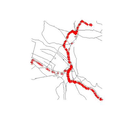
Where the Klass1 roads are in black and the data points are represented in red. With this selection I can now use the function
spsample to create a random grid of points along the road lines:sp.grid.UTM <- spsample(Klass1.cropped,n=1500,type="random")
This generates the following grid, which I think I can share with you in
RData format (gridST.RData): 
As I mentioned, now we need to add a temporal component to this grid. We can do that again using the package spacetime. We first need to create a vector of Date/Times using the function
seq:tm.grid <- seq(as.POSIXct('2011-12-12 06:00 CET'),as.POSIXct('2011-12-14 09:00 CET'),length.out=5)
This creates a vector with 5 elements (
length.out=5), with POSIXct values between the two Date/Times provided. In this case we are interested in creating a spatio-temporal data frame, since we do not yet have any data for it. Therefore we can use the function STF to merge spatial and temporal data into a spatio-temporal grid: grid.ST <- STF(sp.grid.UTM,tm.grid)
This can be used as new data in the kriging function.
Kriging
This is probably the easiest step in the whole process. We have now created the spatio-temporal data frame, compute the best variogram model and create the spatio-temporal prediction grid. All we need to do now is a simple call to the function
krigeST to perform the interpolation:pred <- krigeST(PPB~1, data=timeDF, modelList=sumMetric_Vgm, newdata=grid.ST)
We can plot the results again using the function
stplot:stplot(pred)
More information
There are various tutorial available that offer examples and guidance in performing spatio-temporal kriging. For example we can just write:
vignette("st", package = "gstat")
and a pdf will open with some of the instructions I showed here. Plus there is a demo available at:
demo(stkrige)
In the article “Spatio-Temporal Interpolation using gstat” Gräler et al. explain in details the theory behind spatio-temporal kriging. The pdf of this article can be found here: https://cran.r-project.org/web/packages/gstat/vignettes/spatio-temporal-kriging.pdfThere are also some books and articles that I found useful to better understand the topic, for which I will put the references at the end of the post.
References
Gräler, B., 2012. Different concepts of spatio-temporal kriging [WWW Document]. URL geostat-course.org/system/files/part01.pdf (accessed 8.18.15).Gräler, B., Pebesma, Edzer, Heuvelink, G., 2015. Spatio-Temporal Interpolation using gstat.
Gräler, B., Rehr, M., Gerharz, L., Pebesma, E., 2013. Spatio-temporal analysis and interpolation of PM10 measurements in Europe for 2009.
Oliver, M., Webster, R., Gerrard, J., 1989. Geostatistics in Physical Geography. Part I: Theory. Trans. Inst. Br. Geogr., New Series 14, 259–269. doi:10.2307/622687
Sherman, M., 2011. Spatial statistics and spatio-temporal data: covariance functions and directional properties. John Wiley & Sons.
All the code snippets were created by Pretty R at inside-R.org
This comment has been removed by the author.
ReplyDeleteFor changing the projection of data you wrote
ReplyDelete`ozone.UTM <- spTransform(sub,CRS("+init=epsg:3395")) ` this code.
I found here(http://spatialreference.org/ref/epsg/3395/) that this epsg code is not for Switzerland but you are working with Switzerland (zurich) data. I am woking with South Korea data. Then should I also use this epsg code(3395)? previously I used `sub<- spTransform(sub, CRS("+proj=utm +north +zone=52 +datum=WGS84"))` this code for reprojecting my Korea data. could you please explain little bit what CRS I should use for reprojecting data?
Hi Uzzal
DeleteHow can I know which epsg code my country has?
Hi,
DeleteThank you both for your comments and sorry to Uzzal for the delay in answering.
My data are in Zurich but they are unprojected, meaning that the coordinates are in degrees. That is why I used EPSG=3395.
If you search for Korea on the website you should find what you are looking for:
http://spatialreference.org/ref/?search=korea
This also answers the question from Bibo. To find the EPSG related to your country you can go to http://spatialreference.org and search for the name of the country or the name of the projection system you are using.
I hope this helps,
Fabio
I have a question regarding the output of variogramST, the result has some rows with NA values for np, dist, and gamma. What does this mean?
ReplyDeleteI experienced the same sort of issue when I was preparing the code for the post.
DeleteI concluded that it may be caused by the tunit you are using for the variogram.
For example, if I used "minutes" in the variogram I had the same problem. If the variogram aggregates the data in hours this does not happen, but the variogram computation is more time-consuming.
So correct me if I'm wrong, tunit = "hours" means that If I have data from 7 days, it will combine 7 measurements from each hour in each day? If this is the case then combining them into minutes would take a lot more time, contrary to what I experienced when I replaced "hours" with "mins"..and if I'm reading data of only one day, variogramST would give an error with tunit = "hours" but would work fine with "mins" and results with some NA values in var
DeleteI think that if you have an observation every 10 minutes and you compute the variogram with tunit="hours", R will aggregate the 10 minutes data for each hour in your dataset.
DeleteIf you use tunit="minutes" it will use the actual observations, without aggregating them. That is why the process is faster. However, this may create NAs because there are space-time intervals without observations.
That was my personal conclusion.
Yes I guess this makes sense now. Thanks! this helped a lot! :)
DeleteThis comment has been removed by the author.
ReplyDeleteDear Fabio,
ReplyDeleteThank you for sharing this tutorial. I'm new to spatio-temporal kriging and have a question regarding duplicated points. My data is monthly repeated measurement at exactly same coordinate for each locations. In your post, it was said that kriging cannot handle this issue. Could you please give me any suggestion?
Regards,
Zahra
If the time stamp is different there should not be any problem.
DeleteIt seems that your research is similar to Gräler (2002), which is the first image in the introduction.
If you need any help with the code you can contact me from my website: www.fabioveronesi.net
Excellent tutorial. It is a new content. In my thesis I will work with this content. Very good!
ReplyDeleteGreat Tutorial! I was wondering if if you could attach the data you used here (csv format) ? Thanks
ReplyDeleteHi,
DeleteThe dataset I used is available on the website of the OpenSense project:
http://www.opensense.ethz.ch/trac/wiki/WikiStart
The direct links to 2 free datasets you can use for testing are:
http://www.opensense.ethz.ch/trac/chrome/site/wiki_public/misc/ozon_tram1_14102011_14012012.csv
http://www.opensense.ethz.ch/trac/chrome/site/wiki_public/misc/pm_tram1_14102011_14012012.csv
Best regards,
Fabio
This comment has been removed by the author.
ReplyDeleteHi Fabio,
ReplyDeleteThank you for a great blog which includes all the detail necessary with some good explanations that show your understanding in this. I hit a problem when running the line "projection(data)=CRS("+init=epsg:4326")" as the projection() function doesn't exist in the base library or the ones you listed above. I tried it with proj4string() from the sp library, therefore "proj4string(data)=CRS("+init=epsg:4326")" which seemed to work. Maybe sp has updated since you wrote this blog?
Hi,
DeleteThe function projection is included in the package raster. However, it is just a wrapper for the function proj4string, so your approach is fine.
Hi Fabio,
ReplyDeleteThanks for the great tutorial. I am just starting to use the packages for space -time analysis. Are you able to suggest links to help understanding the graphs produced in the section "Plotting the Variogram"? Is it possible interpret these graphs in terms of spatial temporal autocorrelation? If so, what is the interpretation for the data you present e.g. result of plot(var,map=F)?
Hi Darren,
DeleteThank you for your comment.
I would say the best place to start gathering more information are the references I suggested in the post. Unfortunately, this is still a niche topic so there not much out there in terms of guidelines.
The only thing I can say for interpreting the spatio-temporal autocorrelation is that it is probably better to look at the 3D wireframe. This plot allows us to better observe the relation between time and variograms. With these data for example, we can observe an increase with time of the variogram sill. In other examples, e.g. http://geostat-course.org/system/files/part01.pdf, this is not the case.
I hope this helps you with your research.
Cheers,
Fabio
Hi, could i have your data set? i have some problems, but i think it could be produced by data frame... thanksss!
ReplyDeletePd: do you have some book about spatial-temporal, with repeated measures ?
Hi Fabio,
ReplyDeleteThanks for the useful tutorial! And have you ever surveyed other resource online about Kiring on the roads? Because I wanna know more about value of geospatial point at different time point, like n(location)*m(timing). But I cannot find the more detailed resource, could you do me a favor?
Cheers,
Shako
a great tutorial sir. i have been trying to implement the same on the same dataset as well as on another dataset, but the problem is that the variogramST only executes for 7 percent in some cases, or upto 93 % and stops (finishes) at the same time the var variable will be having only 225 rows and many missing values. what might be the problem . the other dataset iam using has coordinates in the form (41.99549241934282, -87.76960894532459), could it be a problem for this method. another fact about my data is that the coordinates are repeating since it is 10 year period data for each location, and monthly observations are done from may till december.
ReplyDeleteHi
ReplyDeleteIt was a greate tutorial. I have a question about assigning lower, upper and control parameters. How we should choose them?
Also when i select fit.method=7 in fit.stvariogram the error bellow will be appear:
Error in optim(extractPar(model), fitFun, ..., method = method, lower = lower, :
L-BFGS-B needs finite values of 'fn'
Do you know what is the problem?
Thanks alot.
Help, does anyone have a copy of the ozone dataset?
ReplyDeleteIt can't be downloaded anymore from the site
Hi Angie,
DeleteI checked the website and the dataset is still available. You just need to scroll down to the "data" section.
The direct link is: http://www.opensense.ethz.ch/trac/chrome/site/wiki_public/misc/ozon_tram1_14102011_14012012.csv
Regards,
Fabio
Grazie! I am really enjoying this article!
DeleteOne more question please: when I try to print the empirical variogram side to side with the variogram model with "plot(var,separable,map=F)" I only see the separable model. Are there any options I need to check in order to plot in the same way as you did?
Hi Angie,
DeleteI had the same issue recently. I think this function was recently updated.
It may be that now we need to use par
Fabio
Hello! Good tutorial!
ReplyDeleteI have readed your comment about this sentence:
var <- variogramST(PPB~1,data=timeDF,tunit="hours",assumeRegular=F,na.omit=T)
And really the documentation is confusing. You are saying that the variable PPB will be evaluated to compute the spatio temporal variogram, that variable is in the timeDF dataset, and the parameter 'hours' must to coincide with the time unit of the data, that is with the time unit of the slot timeDF@time... Or simply leave it as default, and unit will be catched automatically if it was specified during the construction of the spatio-temporal array (the STIDF class in this case). The idea is to compute correctly the time intervals between observations, specially in this case where the time intervals are not equals...
Regards!
hello, really great post. but I have some trouble. when I run this code in R, that show like this :
ReplyDelete-----
var <- variogramST(PPB~1,data=timeDF,tunit="hours",assumeRegular=F,na.omit=T)
Error in .C("sp_dists", x, y, xx, yy, n, dists, lonlat, PACKAGE = "sp") :
"sp_dists" not available for .C() for package "sp"
----
anyone can help me to solve this problem ?