In some cases we would like to classify the events we have
in our dataset based on their spatial location or on some other data. As an
example we can return to the epidemiological scenario in which we want to
determine if the spread of a certain disease is affected by the presence of a
particular source of pollution. With the G function we are able to determine
quantitatively that our dataset is clustered, which means that the events are
not driven by chance but by some external factor. Now we need to verify that
indeed there is a cluster of points located around the source of pollution, to
do so we need a form of classification of the points.
Cluster analysis refers to a series of techniques that allow
the subdivision of a dataset into subgroups, based on their similarities (James
et al., 2013). There are various clustering method, but probably the most
common is k-means clustering. This technique aims at partitioning the data into
a specific number of clusters, defined a
priori by the user, by minimizing the within-clusters variation. The
within-cluster variation measures how much each event in a cluster k, differs
from the others in the same cluster k. The most common way to compute the
differences is using the squared Euclidean distance (James et al., 2013),
calculated as follow:

Where W_k (I use the underscore to indicate the subscripts) is the within-cluster variation for the cluster k, n_k is the total number of elements in the cluster k, p is the total number of variables we are considering for clustering and x_ij is one variable of one event contained in cluster k. This equation seems complex, but it actually quite easy to understand. To better understand what this means in practice we can take a look at the figure below.
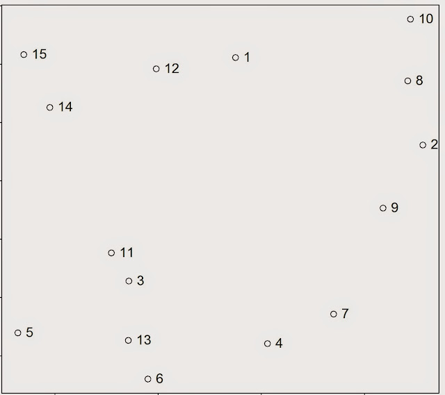
For the sake of the argument we can assume that all the events in this point pattern are located in one unique cluster k, therefore n_k is 15. Since we are clustering events based on their geographical location we are working with two variables, i.e. latitude and longitude; so p is equal to two. To calculate the variance for one single pair of points in cluster k, we simply compute the difference between the first point’s value of the first variable, i.e. its latitude, and the second point value of the same variable; and we do the same for the second variable. So the variance between point 1 and 2 is calculated as follow:
where V_(1:2) is the variance of the two points. Clearly the geographical position is not the only factor that can be used to partition events in a point pattern; for example we can divide earthquakes based on their magnitude. Therefore the two equations can be adapted to take more variables and the only difference is in the length of the linear equation that needs to be solved to calculate the variation between two points. The only problem may be in the number of equations that would need to be solved to obtain a solution. This however is something that the k-means algorithms solves very efficiently.
The algorithm starts by randomly
assigning each event to a cluster, then it calculates the mean centre of each
cluster (we looked at what the mean centre is in the post: Introductory Point Pattern Analysis of Open Crime Data in London). At this point it calculates the Euclidean distance
between each event and the two clusters and reassigns them to a new cluster,
based on the closest mean centre, then it recalculates the mean centres and it
keeps going until the cluster elements stop changing. As an example we can look
at the figure below, assuming we want to divide the events into two clusters.
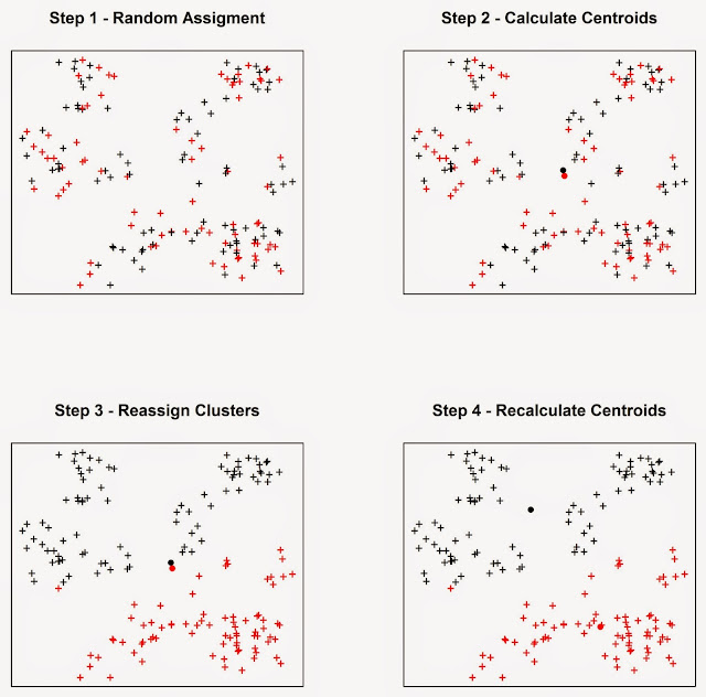
In Step 1
the algorithm assigns each event to a cluster at random. It then
computes the mean centres of the two clusters (Step 2), which are the large
black and red circles. Then the algorithm calculate the Euclidean distance
between each event and the two mean centres, and reassign the events to new
clusters based on the closest mean centre, so if a point was first in cluster
one but it is closer to the mean centre of cluster two it is reassigned to the
latter. Subsequently the mean centres are computed again for the new clusters
(Step 4). This process keeps going until the cluster elements stop changing.
Practical Example
In this experiment we will look at a very simple exercise of cluster analysis of seismic events downloaded from the USGS website. To complete this exercise you would need the following packages: sp, raster, plotrix, rgeos, rgdal and scatterplot3d
I already mentioned in the post Downloading and Visualizing Seismic Events from USGS how to download the open data from the United States Geological Survey, so I will not repeat the process. The code for that is the following.
URL <- "http://earthquake.usgs.gov/earthquakes/feed/v1.0/summary/all_month.csv"
Earthquake_30Days <- read.table(URL, sep = ",", header = T)


#Download, unzip and load the polygon shapefile with the countries' borders
download.file("http://thematicmapping.org/downloads/TM_WORLD_BORDERS_SIMPL-0.3.zip",destfile="TM_WORLD_BORDERS_SIMPL-0.3.zip")
unzip("TM_WORLD_BORDERS_SIMPL-0.3.zip",exdir=getwd())
polygons <- shapefile("TM_WORLD_BORDERS_SIMPL-0.3.shp")
I also included the code to download the shapefile with the borders of all countries.
For the cluster analysis I would like to try to divide the seismic events by origin. In other words I would like to see if there is a way to distinguish between events close to plates, or volcanoes or other faults. In many cases the distinction is hard to make since many volcanoes are originated from subduction, e.g. the Andes, where plates and volcanoes are close to one another and the algorithm may find difficult to distinguish the origins. In any case I would like to explore the use of cluster analysis to see what the algorithm is able to do.
Clearly the first thing we need to do is download data regarding the location of plates, faults and volcanoes. We can find shapefiles with these information at the following website: http://legacy.jefferson.kctcs.edu/techcenter/gis%20data/
The data are provided in zip files, so we need to extract them and load them in R. There are some legal restrictions to use these data. They are distributed by ESRI and can be used in conjunction with the book: "Mapping Our World: GIS Lessons for Educators.". Details of the license and other information may be found here: http://legacy.jefferson.kctcs.edu/techcenter/gis%20data/World/Earthquakes/plat_lin.htm#getacopy
If you have the rights to download and use these data for your studies you can download them directly from the web with the following code. We already looked at code to do this in previous posts so I would not go into details here:
dir.create(paste(getwd(),"/GeologicalData",sep=""))

#Faults
download.file("http://legacy.jefferson.kctcs.edu/techcenter/gis%20data/World/Zip/FAULTS.zip",destfile="GeologicalData/FAULTS.zip")
unzip("GeologicalData/FAULTS.zip",exdir="GeologicalData")

faults <- shapefile("GeologicalData/FAULTS.SHP")


#Plates
download.file("http://legacy.jefferson.kctcs.edu/techcenter/gis%20data/World/Zip/PLAT_LIN.zip",destfile="GeologicalData/plates.zip")
unzip("GeologicalData/plates.zip",exdir="GeologicalData")

plates <- shapefile("GeologicalData/PLAT_LIN.SHP")


#Volcano
download.file("http://legacy.jefferson.kctcs.edu/techcenter/gis%20data/World/Zip/VOLCANO.zip",destfile="GeologicalData/VOLCANO.zip")
unzip("GeologicalData/VOLCANO.zip",exdir="GeologicalData")

volcano <- shapefile("GeologicalData/VOLCANO.SHP")
The only piece of code that I never presented before is the first line, to create a new folder. It is pretty self explanatory, we just need to create a string with the name of the folder and R will create it. The rest of the code downloads data from the address above, unzip them and load them in R.
We have not yet transform the object Earthquake_30Days, which is now a data.frame, into a SpatioPointsDataFrame. The data from USGS contain seismic events that are not only earthquakes but also related to mining and other events. For this analysis we want to keep only the events that are classified as earthquakes, which we can do with the following code:
Earthquakes <- Earthquake_30Days[paste(Earthquake_30Days$type)=="earthquake",]
coordinates(Earthquakes)=~longitude+latitude
This extracts only earthquakes and transform the object into a SpatialObject.
We can create a map that shows the earthquakes alongside all the other geological elements we downloaded using the following code, which saves directly the image in jpeg:
jpeg("Earthquake_Origin.jpg",4000,2000,res=300)
plot(plates,col="red")
plot(polygons,add=T)
title("Earthquakes in the last 30 days",cex.main=3)
lines(faults,col="dark grey")
points(Earthquakes,col="blue",cex=0.5,pch="+")
points(volcano,pch="*",cex=0.7,col="dark red")
legend.pos <- list(x=20.97727,y=-57.86364)

legend(legend.pos,legend=c("Plates","Faults","Volcanoes","Earthquakes"),pch=c("-","-","*","+"),col=c("red","dark grey","dark red","blue"),bty="n",bg=c("white"),y.intersp=0.75,title="Days from Today",cex=0.8)

text(legend.pos$x,legend.pos$y+2,"Legend:")
dev.off()
This code is very similar to what I used here so I will not explain it in details. We just added more elements to the plot and therefore we need to remember that R plots in layers one on top of the other depending on the order in which they appear on the code. For example, as you can see from the code, the first thing we plot are the plates, which will be plotted below everything, even the borders of the polygons, which come second. You can change this just by changing the order of the lines. Just remember to use the option add=T correctly.
The result is the image below:

Before proceeding with the cluster analysis we first need to fix the projections of the SpatialObjects. Luckily the object polygons was created from a shapefile with the projection data attached to it, so we can use it to tell R that the other objects have the same projection:
projection(faults)=projection(polygons)
projection(volcano)=projection(polygons)
projection(Earthquakes)=projection(polygons)
projection(plates)=projection(polygons)
Now we can proceed with the cluster analysis. As I said I would like to try and classify earthquakes based on their distance between the various geological features. To calculate this distance we can use the function gDistance in the package rgeos.
These shapefiles are all unprojected, and their coordinates are in degrees. We cannot use them directly with the function gDistance because it deals only with projected data, so we need to transform them using the function spTransform (in the package rgdal). This function takes two arguments, the first is the SpatialObject, which needs to have projection information, and the second is the data regarding the projection to transform the object into. The code for doing that is the following:
volcanoUTM <- spTransform(volcano,CRS("+init=epsg:3395"))
faultsUTM <- spTransform(faults,CRS("+init=epsg:3395"))
EarthquakesUTM <- spTransform(Earthquakes,CRS("+init=epsg:3395"))
platesUTM <- spTransform(plates,CRS("+init=epsg:3395"))
The projection we are going to use is the standard mercator, details here: http://spatialreference.org/ref/epsg/wgs-84-world-mercator/
NOTE:
the plates object presents lines also along the borders of the image above. This is something that R cannot deal with, so I had to remove them manually from ArcGIS. If you want to replicate this experiment you have to do the same. I do not know of any method in R to do that quickly, if you know it please let me know in the comment section.
We are going to create a matrix of distances between each earthquake and the geological features with the following loop:
distance.matrix <- matrix(0,nrow(Earthquakes),7,dimnames=list(c(),c("Lat","Lon","Mag","Depth","DistV","DistF","DistP")))
for(i in 1:nrow(EarthquakesUTM)){
sub <- EarthquakesUTM[i,]
dist.v <- gDistance(sub,volcanoUTM)
dist.f <- gDistance(sub,faultsUTM)
dist.p <- gDistance(sub,platesUTM)
distance.matrix[i,] <- matrix(c(sub@coords,sub$mag,sub$depth,dist.v,dist.f,dist.p),ncol=7)
}


distDF <- as.data.frame(distance.matrix)
In this code we first create an empty matrix, which is usually wise to do since R already allocates the RAM it would need for the process and it should also be faster to fill it compared to create a new matrix directly from inside the loop. In the loop we iterate through the earthquakes and for each we calculate its distance to the geological features. Finally we change the matrix into a data.frame.
The next step is finding the correct number of clusters. To do that we can follow the approach suggested by Matthew Peeples here: http://www.mattpeeples.net/kmeans.html and also discussed in this stackoverflow post: http://stackoverflow.com/questions/15376075/cluster-analysis-in-r-determine-the-optimal-number-of-clusters
The code for that is the following:
We basically calculate clusters between 2 and 15 and we plot the number of clusters against the "within clusters sum of squares", which is the parameters that is minimized during the clustering process. Generally this quantity decreases very fast up to a point, and then basically stops decreasing. We can see this behaviour from the plot below generated from the earthquake data:

As you can see for 1 and 2 clusters the sum of squares is high and decreases fast, then it decreases between 3 and 5, and then it gets erratic. So probably the best number of clusters would be 5, but clearly this is an empirical method so we would need to check other numbers and test whether they make more sense.
To create the clusters we can simply use the function kmeans, which takes two arguments: the data and the number of clusters:
clust <- kmeans(mydata,5)
distDF$Clusters <- clust$cluster
We can check the physical meaning of the clusters by plotting them against the distance from the geological features using the function scatterplot3d, in the package scatterplot3d:
scatterplot3d(distDF$DistV,xlab="Distance to Volcano",distDF$DistF,ylab="Distance to Fault",distDF$DistP,zlab="Distance to Plate", color = clust$cluster,pch=16,angle=120,scale=0.5,grid=T,box=F)
This function is very similar to the standard plot function, but it takes three arguments instead of just two. I wrote the line of code distinguishing between the three axis to better understand it. So we have the variable for x, and the corresponding axis label, and so on for each axis. Then we set the colours based on clusters, and the symbol with pch, as we would do in plot. The last options are only available here: we have the angle between x and y axis, the scale of the z axis compared to the other two, then we plot a grid on the xy plane and we do not plot a box all around the plot. The result is the following image:

It seems that the red and green cluster are very similar, they differ only because red is closer to volcanoes than faults and vice-versa for the green. The black cluster seems only to be farther away from volcanoes. Finally the blue and light blue clusters seem to be close to volcanoes and far away from the other two features.
We can create an image with the clusters using the following code:
clustSP <- SpatialPointsDataFrame(coords=Earthquakes@coords,data=data.frame(Clusters=clust$cluster))

jpeg("Earthquake_Clusters.jpg",4000,2000,res=300)
plot(plates,col="red")
plot(polygons,add=T)
title("Earthquakes in the last 30 days",cex.main=3)
lines(faults,col="dark grey")
points(volcano,pch="x",cex=0.5,col="yellow")
legend.pos <- list(x=20.97727,y=-57.86364)

points(clustSP,col=clustSP$Clusters,cex=0.5,pch="+")
legend(legend.pos,legend=c("Plates","Faults","Volcanoes"),pch=c("-","-","x","+"),col=c("red","dark grey","yellow"),bty="n",bg=c("white"),y.intersp=0.75,cex=0.6)

text(legend.pos$x,legend.pos$y+2,"Legend:")

dev.off()
I created the object clustSP based on the coordinates in WGS84 so that I can plot everything as before. I also plotted the volcanoes in yellow, so that differ from the red cluster. The result is the following image:

To conclude this experiment I would also like to explore the relation between the distance to the geological features and the magnitude of the earthquakes. To do that we need to identify the events that are at a certain distance from each geological feature. We can use the function gBuffer, again available from the package rgeos, for this job.
This function takes minimum two arguments, the SpatialObject and the maximum distance (in metres because it requires data to be projected) to reach with the buffer, option width. The results is a SpatialPolygons object that include a buffer around the starting features; for example if we start with a point we end up with a circle of radius equal to width. In the code above we first created these buffer areas and then we overlaid EarthquakesUTM with these areas to find the events located within their borders. The overlay function returns two values: NA if the object is outside the buffer area and 1 if it is inside. We can use this information to subset EarthquakesUTM later on.
Now we can include the overlays in EarthquakesUTM as follows:
EarthquakesUTM$volcano <- as.numeric(volcano.over)
EarthquakesUTM$plates  <- as.numeric(plates.over)
EarthquakesUTM$faults  <- as.numeric(faults.over)
To determine if there is a relation between the distance from each feature and the magnitude of the earthquakes we can simply plot the magnitude's distribution for the various events included in the buffer areas we created before with the following code:
plot(density(EarthquakesUTM[paste(EarthquakesUTM$volcano)=="1",]$mag),ylim=c(0,2),xlim=c(0,10),main="Earthquakes by Origin",xlab="Magnitude")
lines(density(EarthquakesUTM[paste(EarthquakesUTM$faults)=="1",]$mag),col="red")
lines(density(EarthquakesUTM[paste(EarthquakesUTM$plates)=="1",]$mag),col="blue")
legend(3,0.6,title="Mean magnitude per origin",legend=c(paste("Volcanic",round(mean(EarthquakesUTM[paste(EarthquakesUTM$volcano)=="1",]$mag),2)),paste("Faults",round(mean(EarthquakesUTM[paste(EarthquakesUTM$faults)=="1",]$mag),2)),paste("Plates",round(mean(EarthquakesUTM[paste(EarthquakesUTM$plates)=="1",]$mag),2))),pch="-",col=c("black","red","blue"),cex=0.8)
which creates the following plot:

It seems that earthquakes close to plates have higher magnitude on average.
R code snippets created by Pretty R at inside-R.org
Hello,
ReplyDeleteWhat is the package for function shapefile ?
Thank you.
This function is part of the package "raster", but it depends on a function in the package "rgdal", so you need to load them both.
DeleteFabio
Great job. I'm running your code right now. Only a suggested, we can use open gis like qgis instead arcgis for delete lines in plate shapefiles.
ReplyDeleteJosé
Fantastic post, hope I can adapt to my data. But when trying to reproduce your example I get an error message when reading SHP files:
ReplyDelete> faults <- shapefile("GeologicalData/FAULTS.shp")
Error: file.exists(extension(x, ".shp")) is not TRUE
The files exist under GeologicalData dir. Which package is needed for this problem? I've got rgdal, raster and shapefiles loaded.
Thanks and best regards
Paco
That error normally means that R cannot find the file.
DeleteAre you sure that in your working directory you have a subdir named GeologicalData?
Fabio
Hi Fabio and thanks for answering. What you suggest was the first I thought. But directory and files do exist. I have also tried to put the full path to GeologicalData but got the same problem.
ReplyDelete> unzip("GeologicalData/FAULTS.zip",exdir="GeologicalData")
> faults <- shapefile("GeologicalData/FAULTS.shp")
Error: file.exists(extension(x, ".shx")) is not TRUE
> faults <- shapefile("./GeologicalData/FAULTS.shp")
Error: file.exists(extension(x, ".shx")) is not TRUE
> faults <- shapefile("/home/meteo/temp/GeologicalData/FAULTS.shp")
Error: file.exists(extension(x, ".shx")) is not TRUE
Paco
I tried myself and it works.
DeleteCould you please create a new script and run the code below (please remember to change the working directory), and then copy and paste what the output of your console?
library(raster)
library(sp)
library(rgdal)
setwd("E:/Temp")
dir.create(paste(getwd(),"/GeologicalData",sep=""))
#Faults
download.file("http://legacy.jefferson.kctcs.edu/techcenter/gis%20data/World/Zip/FAULTS.zip",destfile="GeologicalData/FAULTS.zip")
unzip("GeologicalData/FAULTS.zip",exdir="GeologicalData")
faults <- shapefile("GeologicalData/FAULTS.SHP")
Hi Fabio, I think I've found a solution. Filename extension were in uppercase, the scripts works if they are changed to lowercase. Then I could almost run your script and find the clusters. I have a problem with plates:
ReplyDelete> platesUTM <- spTransform(plates,CRS("+init=epsg:3395"))
non finite transformation detected:
[1] -180 90 Inf Inf
Error in .spTransform_Line(input[[i]], to_args = to_args, from_args = from_args, :
failure in Lines 1 Line 1 points 1
Además: Warning message:
In .spTransform_Line(input[[i]], to_args = to_args, from_args = from_args, :
361 projected point(s) not finite
If I comment plates related lines the script runs fine.
Paco
That's because plates has some lines on the map border for some reason.
DeleteYou need to delete these lines, try this code:
plates$ID <- 1:nrow(plates)
plates <- plates[!plates$ID %in% c(1,4,47,49,51,50,45,6),]
Fabio
Thanks again. Now the point for me is to apply to my data. I have a grid of sea surface temperature values (original .nc files with daily values compiled in lon,lat,SST1,SST2,...SSTn values in an ASCII file). I can't figure out which is the right distance matrix to choose. I want to cluster SST values to find regional patterns for SST across the year. Any suggestion? I'm a little bit lost with statistics as I am not an statician.
DeleteThanks
Please contact me at info[at]fabioveronesi.net with more details about the aim of your experiment and I'll try to help you.
DeleteCheers,
Fabio
Hi Favio, may you re-upload the files which you could find at http://legacy.jefferson.kctcs.edu/techcenter/ ?
ReplyDeleteSite is down unfortunately. Thank you.
I need this file too.
Delete