Showing posts with label Google Maps API. Show all posts

Saturday, 16 February 2019

Geocoding function

This is a very simple function to perform geocoding using the Google Maps API:


getGeoCode <- function(gcStr, key)  {
  library("RJSONIO") #Load Library
  gcStr <- gsub(' ','%20',gcStr) #Encode URL Parameters
  #Open Connection
  connectStr <- paste0('https://maps.googleapis.com/maps/api/geocode/json?address=',gcStr, "&key=",key) 
  con <- url(connectStr)
  data.json <- fromJSON(paste(readLines(con), collapse=""))
  close(con)
  #Flatten the received JSON
  data.json <- unlist(data.json)
  if(data.json["status"]=="OK")   {
    lat <- data.json["results.geometry.location.lat"]
    lng <- data.json["results.geometry.location.lng"]
    gcodes <- c(lat, lng)
    names(gcodes) <- c("Lat", "Lng")
    return (gcodes)
  }
}

Essentially, users need to get an API key from google and then use as an input (string) for the function. The function itself is very simple, and it is an adaptation of some code I found on-line (unfortunately I did not write down where I found the original version so I do not have a way to reference the source, sorry!!).


geoCodes <- getGeoCode(gcStr="11 via del piano, empoli", key)

To use the function we simply need to include an address, and it will return its coordinates in WGS84.
It can be used in a mutate call within dplyr and it is reasonably fast.

The repository is here:
https://github.com/fveronesi/RGeocode.r

Sunday, 21 June 2015

Organize a walk around London with R

The subtitle of this post can be "How to plot multiple elements on interactive web maps in R".
In this experiment I will show how to include multiple elements in interactive maps created using both plotGoogleMaps and leafletR. To complete the work presented here you would need the following packages: sp, raster, plotGoogleMaps and leafletR.

I am going to use data from the OpenStreet maps, which can be downloaded for free from this website: weogeo.com
In particular I downloaded the shapefile with the stores, the one with the tourist attractions and the polyline shapefile with all the roads in London. I will assume that you want to spend a day or two walking around London, and for this you would need the location of some hotels and the locations of all the Greggs in the area, for lunch. You need to create a web map that you can take with you when you walk around the city with all these customized elements, that's how you create it.

Once you have downloaded the shapefile from weogeo.com you can open them and assign the correct projection with the following code:

stores <- shapefile("weogeo_j117529/data/shop_point.shp")
projection(stores)=CRS("+init=epsg:3857")
 
roads <- shapefile("weogeo_j117529/data/route_line.shp")
projection(roads)=CRS("+init=epsg:3857")
 
tourism <- shapefile("weogeo_j117529/data/tourism_point.shp")
projection(tourism)=CRS("+init=epsg:3857")

To extract only the data we would need to the map we can use these lines:

Greggs <- stores[stores$NAME %in% c("Gregg's","greggs","Greggs"),]
 
Hotel <- tourism[tourism$TOURISM=="hotel",]
Hotel <- Hotel[sample(1:nrow(Hotel),10),]
 
 
Footpaths <- roads[roads$ROUTE=="foot",]


plotGoogleMaps
I created three objects, two are points (Greggs and Hotel) and the last is of class SpatialLinesDataFrame. We already saw how to plot Spatial objects with plotGoogleMaps, here the only difference is that we need to create several maps and then link them together.
Let's take a look at the following code:

Greggs.google <- plotGoogleMaps(Greggs,iconMarker=rep("http://local-insiders.com/wp-content/themes/localinsiders/includes/img/tag_icon_food.png",nrow(Greggs)),mapTypeId="ROADMAP",add=T,flat=T,legend=F,layerName="Gregg's",fitBounds=F,zoom=13)
Hotel.google <- plotGoogleMaps(Hotel,iconMarker=rep("http://www.linguistics.ucsb.edu/projects/weal/images/hotel.png",nrow(Hotel)),mapTypeId="ROADMAP",add=T,flat=T,legend=F,layerName="Hotels",previousMap=Greggs.google)
 
plotGoogleMaps(Footpaths,col="dark green",mapTypeId="ROADMAP",filename="Multiple_Objects_GoogleMaps.html",legend=F,previousMap=Hotel.google,layerName="Footpaths",strokeWeight=2)

As you can see I first create two objects using the same function and then I call again the same function to draw and save the map. I can link the three maps together using the option add=T and previousMap.
We need to be careful here though, because the use of the option add is different from the standard plot function. In plot I can call the first and then if I want to add a second I call again the function with the option add=T. Here this option needs to go in the first and second calls, not in the last. Basically in this case we are saying to R not to close the plot because later on we are going to add elements to it. In the last line we do not put add=T, thus saying to R to go ahead and close the plot.

Another important option is previousMap, which is used starting from the second plot to link the various elements. This option is used referencing the previous object, meaning that I reference the map in Hotel.google to the map map to Greggs.google, while in the last call I reference it to the previous Hotel.google, not the very first.

The zoom level, if you want to set it, goes only in the first plot.

Another thing I changed compared to the last example is the addition of custom icons to the plot, using the option iconMarker. This takes a vector of icons, not just one, with the same length of the SpatialObject to be plotted. That is why I use the function rep, to create a vector with the same URL repeated for a number of times equal to the length of the object.
The icon can be whatever image you like. You can find a collection of free icons from this website: http://kml4earth.appspot.com/icons.html

The result is the map below, available here: Multiple_Objects_GoogleMaps.html


leafletR
We can do the same thing using leafletR. We first need to create GeoJSON files for each element of the map using the following lines:

Greggs.geojson <- toGeoJSON(Greggs)
Hotel.geojson <- toGeoJSON(Hotel)
Footpaths.geojson <- toGeoJSON(Footpaths)

Now we need to set the style for each element. For this task we are going to use the function styleSingle, which basically defines a single style for all the elements of the GeoJSON. This differ from the map in a previous post in which we used the function styleGrad to create graduated colors depending of certain features of the dataset.
We can change the icons of the elements in leafletR using the following code:

Greggs.style <- styleSingle(marker=c("fast-food", "red", "s"))
Hotel.style <- styleSingle(marker=c("lodging", "blue", "s"))
Footpaths.style <- styleSingle(col="darkred",lwd=4)

As you can see we have the option marker that takes a vector with the name of the icon, its color and its size (between "s" for small, "m" for medium and "l" for large). The names of the icons can be found here: https://www.mapbox.com/maki/, where you have a series of icons and if you hover the mouse over them you would see some info, among which there is the name to use here, as the very last name. The style of the lines is set using the two options col and lwd, for line width.

Then we can simply use the function leaflet to set the various elements and styles of the map:

leaflet(c(Greggs.geojson,Hotel.geojson,Footpaths.geojson),style=list(Greggs.style,Hotel.style,Footpaths.style),popup=list(c("NAME"),c("NAME"),c("OPERATOR")),base.map="osm")

The result is the image below and the map available here: http://www.fabioveronesi.net/Blog/map.html


R code snippets created by Pretty R at inside-R.org

Thursday, 28 May 2015

Live Earthquake Map with Shiny and Google Map API

In the post Exchange data between R and the Google Maps API using Shiny I presented a very simple way to allow communication between R and javascript using Shiny.

This is an example of a practical approach for which the same system can be used. Here I created a tool to visualize seismic events, collected from USGS, in the Google Maps API using R to do some basic data preparation. The procedure to complete this experiment is pretty much identical to what I presented in the post mentioned above, so I will not repeated here.


The final map looks like this:


and it is accessible from this site, hosted on the Amazon Cloud: Earthquake

The colours of the markers depends on magnitude and they are set in R. For magnitudes below 2 the marker is green, between 2 and 4 is yellow, between 4 and 6 is orange and above 6 is red.
I also set R to export other information about the event to the json file that I then use to populate the infowindow of each marker.

The code for creating this map consists of two pieces, an index.html file (which needs to go in a folder names www) and the file server.r, available below:

Server.r
 # server.R  
 #Title: Earthquake Visualization in Shiny  
 #Copyright: Fabio Veronesi  
   
 library(sp)  
 library(rjson)  
 library(RJSONIO)  
   
    
 shinyServer(function(input, output) {  
   
 output$json <- reactive ({  
 if(length(input$Earth)>0){  
 if(input$Earth==1){  
 hour <- read.table("http://earthquake.usgs.gov/earthquakes/feed/v1.0/summary/all_hour.csv", sep = ",", header = T)  
 if(nrow(hour)>0){  
 lis <- list()  
 for(i in 1:nrow(hour)){  
   
 if(hour$mag[i]<=2){icon="http://maps.gstatic.com/mapfiles/ridefinder-images/mm_20_green.png"}  
 else if(hour$mag[i]>2&hour$mag[i]<=4){icon="http://maps.gstatic.com/mapfiles/ridefinder-images/mm_20_yellow.png"}  
 else if(hour$mag[i]>4&hour$mag[i]<=6){icon="http://maps.gstatic.com/mapfiles/ridefinder-images/mm_20_orange.png"}  
 else {icon="http://maps.gstatic.com/mapfiles/ridefinder-images/mm_20_red.png"}  
   
 Date.hour <- substring(hour$time[i],1,10)  
 Time.hour <- substring(hour$time[i],12,23)  
   
 lis[[i]] <- list(i,hour$longitude[i],hour$latitude[i],icon,hour$place[i],hour$depth[i],hour$mag[i],Date.hour,Time.hour)  
 }  
   
   
 #This code creates the variable test directly in javascript for export the grid in the Google Maps API  
 #I have taken this part from:http://stackoverflow.com/questions/26719334/passing-json-data-to-a-javascript-object-with-shiny  
    paste('<script>test=',         
       RJSONIO::toJSON(lis),        
       ';setAllMap();Cities_Markers();',        
       '</script>')  
 }  
 }  
   
 else if(input$Earth==4){  
 month <- read.table("http://earthquake.usgs.gov/earthquakes/feed/v1.0/summary/all_month.csv", sep = ",", header = T)  
 if(nrow(month)>0){  
 lis <- list()  
 for(i in 1:nrow(month)){  
   
 if(month$mag[i]<=2){icon="http://maps.gstatic.com/mapfiles/ridefinder-images/mm_20_green.png"}  
 else if(month$mag[i]>2&month$mag[i]<=4){icon="http://maps.gstatic.com/mapfiles/ridefinder-images/mm_20_yellow.png"}  
 else if(month$mag[i]>4&month$mag[i]<=6){icon="http://maps.gstatic.com/mapfiles/ridefinder-images/mm_20_orange.png"}  
 else {icon="http://maps.gstatic.com/mapfiles/ridefinder-images/mm_20_red.png"}  
   
 Date.month <- substring(month$time[i],1,10)  
 Time.month <- substring(month$time[i],12,23)  
   
 lis[[i]] <- list(i,month$longitude[i],month$latitude[i],icon,month$place[i],month$depth[i],month$mag[i],Date.month,Time.month)  
 }  
   
   
 #This code creates the variable test directly in javascript for export the grid in the Google Maps API  
 #I have taken this part from:http://stackoverflow.com/questions/26719334/passing-json-data-to-a-javascript-object-with-shiny  
    paste('<script>test=',         
       RJSONIO::toJSON(lis),        
       ';setAllMap();Cities_Markers();',        
       '</script>')  
 }  
 }  
   
   
 else if(input$Earth==3){  
 week <- read.table("http://earthquake.usgs.gov/earthquakes/feed/v1.0/summary/all_week.csv", sep = ",", header = T)  
 if(nrow(week)>0){  
 lis <- list()  
 for(i in 1:nrow(week)){  
   
 if(week$mag[i]<=2){icon="http://maps.gstatic.com/mapfiles/ridefinder-images/mm_20_green.png"}  
 else if(week$mag[i]>2&week$mag[i]<=4){icon="http://maps.gstatic.com/mapfiles/ridefinder-images/mm_20_yellow.png"}  
 else if(week$mag[i]>4&week$mag[i]<=6){icon="http://maps.gstatic.com/mapfiles/ridefinder-images/mm_20_orange.png"}  
 else {icon="http://maps.gstatic.com/mapfiles/ridefinder-images/mm_20_red.png"}  
   
 Date.week <- substring(week$time[i],1,10)  
 Time.week <- substring(week$time[i],12,23)  
   
 lis[[i]] <- list(i,week$longitude[i],week$latitude[i],icon,week$place[i],week$depth[i],week$mag[i],Date.week,Time.week)  
 }  
   
   
 #This code creates the variable test directly in javascript for export the grid in the Google Maps API  
 #I have taken this part from:http://stackoverflow.com/questions/26719334/passing-json-data-to-a-javascript-object-with-shiny  
    paste('<script>test=',         
       RJSONIO::toJSON(lis),        
       ';setAllMap();Cities_Markers();',        
       '</script>')  
 }  
 }  


 else {  
 day <- read.table("http://earthquake.usgs.gov/earthquakes/feed/v1.0/summary/all_day.csv", sep = ",", header = T)  
 if(nrow(day)>0){  
 lis <- list()  
 for(i in 1:nrow(day)){  
   
 if(day$mag[i]<=2){icon="http://maps.gstatic.com/mapfiles/ridefinder-images/mm_20_green.png"}  
 else if(day$mag[i]>2&day$mag[i]<=4){icon="http://maps.gstatic.com/mapfiles/ridefinder-images/mm_20_yellow.png"}  
 else if(day$mag[i]>4&day$mag[i]<=6){icon="http://maps.gstatic.com/mapfiles/ridefinder-images/mm_20_orange.png"}  
 else {icon="http://maps.gstatic.com/mapfiles/ridefinder-images/mm_20_red.png"}  
   
 Date.day <- substring(day$time[i],1,10)  
 Time.day <- substring(day$time[i],12,23)  
   
 lis[[i]] <- list(i,day$longitude[i],day$latitude[i],icon,day$place[i],day$depth[i],day$mag[i],Date.day,Time.day)  
 }  
   
   
 #This code creates the variable test directly in javascript for export the grid in the Google Maps API  
 #I have taken this part from:http://stackoverflow.com/questions/26719334/passing-json-data-to-a-javascript-object-with-shiny  
    paste('<script>test=',         
       RJSONIO::toJSON(lis),        
       ';setAllMap();Cities_Markers();',        
       '</script>')  
 }  
 }  
 }  
 })  
 })  


Index.html
 <!DOCTYPE html>  
 <html>  
 <head>  
 <title>Earthquake Visualization in Shiny</title>  
   
 <!--METADATA-->    
 <meta name="author" content="Fabio Veronesi">  
 <meta name="copyright" content="©Fabio Veronesi">  
 <meta http-equiv="Content-Language" content="en-gb">  
 <meta charset="utf-8"/>  
   
 <style type="text/css">  
   
 html { height: 100% }  
 body { height: 100%; margin: 0; padding: 0 }  
 map-canvas { height: 100%; width:100% }  
   
 .btn {  
  background: #dde6d8;  
  background-image: -webkit-linear-gradient(top, #dde6d8, #859ead);  
  background-image: -moz-linear-gradient(top, #dde6d8, #859ead);  
  background-image: -ms-linear-gradient(top, #dde6d8, #859ead);  
  background-image: -o-linear-gradient(top, #dde6d8, #859ead);  
  background-image: linear-gradient(to bottom, #dde6d8, #859ead);  
  -webkit-border-radius: 7;  
  -moz-border-radius: 7;  
  border-radius: 7px;  
  font-family: Arial;  
  color: #000000;  
  font-size: 20px;  
  padding: 9px 20px 10px 20px;  
  text-decoration: none;  
 }  
   
 .btn:hover {  
  background: #f29f9f;  
  background-image: -webkit-linear-gradient(top, #f29f9f, #ab1111);  
  background-image: -moz-linear-gradient(top, #f29f9f, #ab1111);  
  background-image: -ms-linear-gradient(top, #f29f9f, #ab1111);  
  background-image: -o-linear-gradient(top, #f29f9f, #ab1111);  
  background-image: linear-gradient(to bottom, #f29f9f, #ab1111);  
  text-decoration: none;  
 }  
   
 </style>  
   
        
 <script type="text/javascript" src="http://google-maps-utility-library-v3.googlecode.com/svn/tags/markerclusterer/1.0/src/markerclusterer.js"></script>  
   
 <script src="https://maps.googleapis.com/maps/api/js?v=3.exp&signed_in=true&libraries=drawing"></script>  
   
 <script type="application/shiny-singletons"></script>  
 <script type="application/html-dependencies">json2[2014.02.04];jquery[1.11.0];shiny[0.11.1];ionrangeslider[2.0.2];bootstrap[3.3.1]</script>  
 <script src="shared/json2-min.js"></script>  
 <script src="shared/jquery.min.js"></script>  
 <link href="shared/shiny.css" rel="stylesheet" />  
 <script src="shared/shiny.min.js"></script>  
 <link href="shared/ionrangeslider/css/normalize.css" rel="stylesheet" />  
 <link href="shared/ionrangeslider/css/ion.rangeSlider.css" rel="stylesheet" />  
 <link href="shared/ionrangeslider/css/ion.rangeSlider.skinShiny.css" rel="stylesheet" />  
 <script src="shared/ionrangeslider/js/ion.rangeSlider.min.js"></script>  
 <link href="shared/bootstrap/css/bootstrap.min.css" rel="stylesheet" />  
 <script src="shared/bootstrap/js/bootstrap.min.js"></script>  
 <script src="shared/bootstrap/shim/html5shiv.min.js"></script>  
 <script src="shared/bootstrap/shim/respond.min.js"></script>  
   
        
      <script type="text/javascript">  
      var map = null;  
      var Gmarkers = [];  
        
   
      function Cities_Markers() {  
             
           var infowindow = new google.maps.InfoWindow({ maxWidth: 500,maxHeight:500 });  
   
           //Loop to add markers to the map based on the JSON exported from R, which is within the variable test  
           for (var i = 0; i < test.length; i++) {   
                var lat = test[i][2]  
                var lng = test[i][1]  
                var marker = new google.maps.Marker({  
                     position: new google.maps.LatLng(lat, lng),  
                     title: 'test',  
                     map: map,  
                     icon:test[i][3]  
                });  
             
           //This sets up the infowindow  
           google.maps.event.addListener(marker, 'click', (function(marker, i) {  
                return function() {  
                     infowindow.setContent('<div id="content"><p><b>Location</b> = '+  
                     test[i][4]+'<p>'+  
                     '<b>Depth</b> = '+test[i][5]+'Km <p>'+  
                     '<b>Magnitude</b> = '+test[i][6]+ '<p>'+  
                     '<b>Date</b> = '+test[i][7]+'<p>'+  
                     '<b>Time</b> = '+test[i][8]+'</div>');  
                     infowindow.open(map, marker);  
                }  
                })(marker, i));  
           Gmarkers.push(marker);  
           };  
             
   
      };  
   
      //Function to remove all the markers from the map  
      function setAllMap() {  
           for (var i = 0; i < Gmarkers.length; i++) {  
                Gmarkers[i].setMap(null);  
           }  
 }  
        
      //Initialize the map  
      function initialize() {  
           var mapOptions = {  
           center: new google.maps.LatLng(31.6, 0),  
           zoom: 3,  
           mapTypeId: google.maps.MapTypeId.TERRAIN  
      };  
   
      map = new google.maps.Map(document.getElementById('map-canvas'),mapOptions);  
        
    
 }  
   
   
 google.maps.event.addDomListener(window, 'load', initialize);  
   </script>  
        
   
 </head>  
   
   
 <body>  
   
  <div id="json" class="shiny-html-output"></div>  
   
    
  <button type="button" class="btn" id="hour" onClick="Shiny.onInputChange('Earth', 1)" style="position:absolute;top:1%;left:1%;width:100px;z-index:999">Last Hour</button>  
  <button type="button" class="btn" id="day" onClick="Shiny.onInputChange('Earth', 2)" style="position:absolute;top:1%;left:10%;width:100px;z-index:999">Last Day</button>  
  <button type="button" class="btn" id="week" onClick="Shiny.onInputChange('Earth', 3)" style="position:absolute;top:1%;left:20%;width:100px;z-index:999">Last Week</button>  
  <button type="button" class="btn" id="month" onClick="Shiny.onInputChange('Earth', 4)" style="position:absolute;top:1%;left:30%;width:100px;z-index:999">Last Month</button>  
    
  <div id="map-canvas" style="top:0%;right:0%;width:100%;height:100%;z-index:1"></div>  


 </body>  
 </html>  
Created with CodeFormatter

Monday, 25 May 2015

Interactive maps of Crime data in Greater London

In the previous post we looked at ways to perform some introductory point pattern analysis of open data downloaded from Police.uk. As you remember we subset the dataset of crimes in the Greater London area, extracting only the drug related ones. Subsequently, we looked at ways to use those data with the package spatstat and perform basic statistics.
In this post I will briefly discuss ways to create interactive plots of the results of the point pattern analysis using the Google Maps API and Leaflet from R.

Number of Crimes by Borough
In the previous post we looped through the GreaterLondonUTM shapefile to extract the area of each borough and then counted the number of crimes within its border. To show the results we used a simple barplot. Here I would like to use the same method I presented in my post Interactive Maps for the Web to plot these results on Google Maps.

This post is intended to be a continuation of the previous, so I will not present again the methods and objects we used in the previous experiment. To make this code work you can just copy and paste it below the code you created before and it should work just fine.

First of all, let's create a new object including only the names of the boroughs from the GreaterLondonUTM shapefile. We need to do this because otherwise when we will click on a polygons on the map it will show us a long list of useless data.

GreaterLondon.Google <- GreaterLondonUTM[,"name"]

The new object has only one column with the name of each borough.
Now we can create a loop to iterate through these names and calculate the intensity of the crimes:

Borough <- GreaterLondonUTM[,"name"]
 
for(i in unique(GreaterLondonUTM$name)){
sub.name <- Local.Intensity[Local.Intensity[,1]==i,2]
 
Borough[Borough$name==i,"Intensity"] <- sub.name
 
Borough[Borough$name==i,"Intensity.Area"] <- round(sub.name/(GreaterLondonUTM[GreaterLondonUTM$name==i,]@polygons[[1]]@area/10000),4)
}

As you can see this loop selects one name at the time, then subset the object Local.Intensity (which we created in the previous post) to extract the number of crimes for each borough. The next line attach this intensity to the object Borough as a new column named Intensity. However, the code does not stop here. We also create another column named Intensity.Area in which we calculate the amount of crimes per unit area. Since the area from the shapefile is in square meters and the number were very high, I though about dividing it by 10'000 in order to have a unit area of 10 square km. So this column shows the amount of crime per 10 square km in each borough. This should correct the fact that certain borough have a relatively high number of crimes only because their area is larger than others.

Now we can use again the package plotGoogleMaps to create a beautiful visualization of our results and save it in HTML so that we can upload it to our website or blog.
The code for doing that is very simple and it is presented below:

plotGoogleMaps(Borough,zcol="Intensity",filename="Crimes_Boroughs.html",layerName="Number of Crimes", fillOpacity=0.4,strokeWeight=0,mapTypeId="ROADMAP")

I decided to plot the polygons on top of the roadmap and not on top of the satellite image, which is the default for the function. Thus I added the option mapTypeId="ROADMAP".
The result is the map shown below and at this link: Crimes on GoogleMaps


In the post Interactive Maps for the Web in R I received a comment from Gerardo Celis, whom I thank for it, telling me that now in R is also available the package leafletR, that allows us to create interactive maps based on Leaflet. So for this new experiment I decided to try it out!

I started from the sample of code presented here: https://github.com/chgrl/leafletR and I adapted with very few changes to my data.
The function leaflet does not work directly with Spatial data, we first need to transform them into GeoJSON with another function in leafletR:

Borough.Leaflet <- toGeoJSON(Borough)

Extremely simple!!

Now we need to set the style to use for plotting the polygons using the function styleGrad, which is used to create a list of colors based on a particular attribute:

map.style <- styleGrad(pro="Intensity",breaks=seq(min(Borough$Intensity),max(Borough$Intensity)+15,by=20),style.val=cm.colors(10),leg="Number of Crimes", fill.alpha=0.4, lwd=0)

In this function we need to set several options:
pro = is the name of the attribute (as the column name) to use for setting the colors
breaks = this option is used to create the ranges of values for each colors. In this case, as in the example, I just created a sequence of values from the minimum to the maximum. As you can see from the code I added 15 to the maximum value. This is because the number of breaks needs to have 1 more element compared to the number of colors. For example, if we set 10 breaks we would need to set 9 colors. For this reason if the sequence of breaks ends before the maximum, the polygons with the maximum number of crimes would be presented in grey.
This is important!!

style.val = this option takes the color scale to be used to present the polygons. We can select among one of the default scales or we can create a new one with the function color.scale in the package plotrix, which I already discussed here: Downloading and Visualizing Seismic Events from USGS

leg = this is simply the title of the legend
fill.alpha = is the opacity of the colors in the map (ranges from 0 to 1, where 1 is the maximum)
lwd =  is the width of the line between polygons

After we set the style we can simply call the function leaflet to create the map:

leaflet(Borough.Leaflet,popup=c("name","Intensity","Intensity.Area"),style=map.style)

In this function we need to input the name of the GeoJSON object we created before, the style of the map and the names of the columns to use for the popups.
The result is the map shown below and available at this link: Leaflet Map


I must say this function is very neat. First of all the function plotGoogleMaps, if you do not set the name of the HTML file, creates a series of temporary files stored in your temp folder, which is not great. Then even if you set the name of the file the legend is saved into different image files every time you call the function, which you may do many times until you are fully satisfied the result.
The package leafletR on the other hand creates a new folder inside the working directory where it stores both the GeoJSON and the HTML file, and every time you modify the visualization the function overlays the same file.
However, I noticed that I cannot see the map if I open the HTML files from my PC. I had to upload the file to my website every time I changed it to actually see these changes and how they affected the plot. This may be something related to my PC, however.


Density of Crimes in raster format
As you may remember from the previous post, one of the steps included in a point pattern analysis is the computation of the spatial density of the events. One of the techniques to do that is the kernel density, which basically calculates the density continuously across the study area, thus creating a raster.
We already looked at the kernel density in the previous post so I will not go into details here, the code for computing the density and transform it into a raster is the following:

Density <- density.ppp(Drugs.ppp, sigma = 500,edge=T,W=as.mask(window,eps=c(100,100)))
Density.raster <- raster(Density)
projection(Density.raster)=projection(GreaterLondonUTM)

The first lines is basically the same we used in the previous post. The only difference is that here I added the option W to set the resolution of the map with eps at 100x100 m.
Then I simply transformed the first object into a raster and assign to it the same UTM projection of the object GreaterLondonUTM.
Now we can create the map. As far as I know (and for what I tested) leafletR is not yet able to plot raster objects, so the only way we have of doing it is again to use the function plotGoogleMaps:

plotGoogleMaps(Density.raster,filename="Crimes_Density.html",layerName="Number of Crimes", fillOpacity=0.4,strokeWeight=0,colPalette=rev(heat.colors(10)))

When we use this function to plot a raster we clearly do not need to specify the zcol option. Moreover, here I changed the default color scale using the function colPalette to a reverse heat.colors, which I think is more appropriate for such a map. The result is the map below and at this link: Crime Density


Density of Crimes as contour lines
The raster presented above can also be represented as contour lines. The advantage of this type of visualization is that it is less intrusive, compared to a raster, and can also be better suited to pinpoint problematic locations.
Doing this in R is extremely simple, since there is a dedicated function in the package raster:

Contour <- rasterToContour(Density.raster,maxpixels=100000,nlevels=10)

This function transforms the raster above into a series of 10 contour lines (we can change the number of lines by changing the option nlevels).

Now we can plot these lines to an interactive web map. I first tested again the use of plotGoogleMaps but I was surprised to see that for contour lines it does not seem to do a good job. I do not fully know the reason, but if I use the object Contour with this function it does not plot all the lines on the Google map and therefore the visualization is useless.
For this reason I will present below the lines to plot contour lines using leafletR:

Contour.Leaflet <- toGeoJSON(Contour)
 
colour.scale <- color.scale(1:(length(Contour$level)-1),color.spec="rgb",extremes=c("red","blue"))
map.style <- styleGrad(pro="level",breaks=Contour$level,style.val=colour.scale,leg="Number of Crimes", lwd=2)
leaflet(Contour.Leaflet,style=map.style,base.map="tls")

As mentioned, the first thing to do to use leafletR is to transform our Spatial object into a GeoJSON; the object Contour belongs to the class SpatialLinesDataFrame, so it is supported in the function toGeoJSON.
The next step is again to set the style of the map and then plot it. In this code I changed a few things just to show some more options. The first thing is the custom color scale I created using the function color.scale in the package plotrix. The only thing that the function styleGrad needs to set the colors in the option style.val is a vector of colors, which must be long one unit less than the vector used for the breaks. In this case the object Contour has only one property, namely "level", which is a vector of class factor. The function styleGrad can use it to create the breaks but the function color.scale cannot use it to create the list of colors. We can work around this problem by setting the length of the color.scale vector using another vector: 1:(length(Contour$level)-1, which basically creates a vector of integers from 1 to the length of Contours minus one. The result of this function is a vector of colors ranging from red to blue, which we can plug in in the following function.
In the function leaflet the only thing I changed is the base.map option, in which I use "tls". From the help page of the function we can see that the following options are available:

"One or a list of "osm" (OpenStreetMap standard map), "tls" (Thunderforest Landscape), "mqosm" (MapQuest OSM), "mqsat" (MapQuest Open Aerial),"water" (Stamen Watercolor), "toner" (Stamen Toner), "tonerbg" (Stamen Toner background), "tonerlite" (Stamen Toner lite), "positron" (CartoDB Positron) or "darkmatter" (CartoDB Dark matter). "

These lines create the following image, available as a webpage here: Contour


R code snippets created by Pretty R at inside-R.org

Friday, 15 May 2015

Interactive maps for the web in R

Static Maps
In the last post I showed how to download economic data from the World Bank's website and create choropleth maps in R (Global Economic Maps).
In this post I want to focus more on how to visualize those maps.

Sp Package
Probably the simplest way of plotting choropleth maps in R is the one I showed in the previous post, using the function ssplot(). For example with a call like the following:

library(sp)
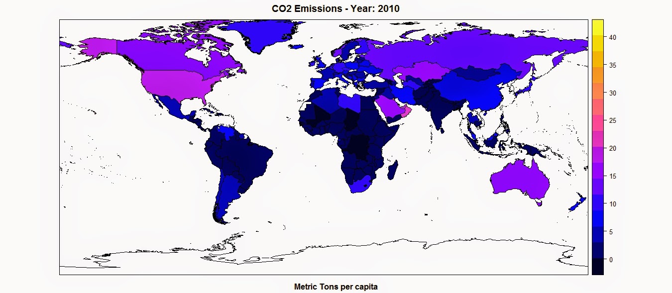
spplot(polygons,"CO2",main=paste("CO2 Emissions - Year:",CO2.year),sub="Metric Tons per capita")

This function takes the object polygons, which is a SpatialPolygonsDataFrame, and in quotations marks the name of the column where to find the values to assign, as colors, to each polygon. This are two basic mandatory elements to call the function. However, we can increase the information in the plot by adding additional elements, such as a title, option main, and a sub title, option sub.

This function creates the following plot:

The color scale is selected automatically and can be changed with a couple of standard functions or using customized color scales. For more information please refer to this page: http://rstudio-pubs-static.s3.amazonaws.com/7202_3145df2a90a44e6e86a0637bc4264f9f.html


Standard Plot
Another way of plotting maps is by using the standard plot() function, which allows us to increase the flexibility of the plot, for example by customizing the position of the color legend.
The flip side is that, since it is the most basic plotting function available and it does not have many built-in options, this function require more lines of code to achieve a good result.
Let's take a look at the code below:

library(plotrix)
CO2.dat <- na.omit(polygons$CO2)
colorScale <- color.scale(CO2.dat,color.spec="rgb",extremes=c("red","blue"),alpha=0.8)
 
colors.DF <- data.frame(CO2.dat,colorScale)
colors.DF <- colors.DF[with(colors.DF, order(colors.DF[,1])), ]
colors.DF$ID <- 1:nrow(colors.DF)
breaks <- seq(1,nrow(colors.DF),length.out=10)
 
 
jpeg("CO2_Emissions.jpg",7000,5000,res=300)
plot(polygons,col=colorScale)
title("CO2 Emissions",cex.main=3)
 
legend.pos <- list(x=-28.52392,y=-20.59119)
legendg(legend.pos,legend=c(round(colors.DF[colors.DF$ID %in% round(breaks,0),1],2)),fill=paste(colors.DF[colors.DF$ID %in% round(breaks,0),2]),bty="n",bg=c("white"),y.intersp=0.75,title="Metric tons per capita",cex=0.8) 
 
dev.off()


By simpling calling the plot function with the object polygons, R is going to create an image of the country borders with no filling. If we want to add colors to the plot we first need to create a color scale using our data. To do so we can use the function color.scale() in the package plotrix, which I used also in the post regarding the visualization seismic events from USGS (Downloading and Visualizing Seismic Events from USGS ). This function takes a vector, plus the color of the extremes of the color scale, in this case red and blue, and creates a vector of intermediate colors to assign to each element of the data vector.
In this example I first created a vector named CO2.dat, with the values of CO2 for each polygon, excluding NAs. Then I feed it to the color.scale() function.

The next step is the creation of the legend. The first step is the creation of the breaks we are going to need to present the full spectrum of colors used in the plot. For this I first created a data.frame with values and colors and then I subset it into 10 elements, which is the length of the legend.
Now we can submit the rest of the code to create a plot and the legend and save it into the jpeg file below:


Interactive Maps
The maps we created thus far are good for showing our data on papers and allow the reader to have a good understanding of what we are trying to show with them. Clearly these are not the only two methods available to create maps in R, many more are available. In particular ggplot2 now features ways of creating beautiful static maps. For more information please refer to these website and blog posts:
Maps in R
Making Maps in R
Introduction to Spatial Data and ggplot2
Plot maps like a boss
Making Maps with R

In this post however, I would like to focus on ways to move away from static maps and embrace the fact that we are now connected to the web all the times. This allow us to create maps specifically design for the web, which can also be much more easy to read by the general public that is used to them.
These sort of maps are the interactive maps that we see all over the web, for example from Google. These are created in javascript and are extremely powerful. The problem is, we know R and we work on it all the time, but we do not necessarily know how to code in javascript. So how can we create beautiful interactive maps for the web if we cannot code in javascript and HTML?

Luckily for us developers have create packages that allow us to create maps using standard R code but n the form of HTML page that we can upload directly on our website. I will now examine the packages I know and use regularly for plotting choropleth maps.


googleVis
This package is extremely simple to use and yet capable of creating beautiful maps that can be uploaded easily to our website.
Let's look at the code below:

data.poly <- as.data.frame(polygons)
data.poly <- data.poly[,c(5,12)]
names(data.poly) <- c("Country Name","CO2 emissions (metric tons per capita)")
 
map <- gvisGeoMap(data=data.poly, locationvar = "Country Name", numvar='CO2 emissions (metric tons per capita)',options=list(width='800px',heigth='500px',colors="['0x0000ff', '0xff0000']"))
plot(map)
 
print(map,file="Map.html")
 
#http://www.javascripter.net/faq/rgbtohex.htm
#To find HEX codes for RGB colors

The first thing to do is clearly to load the package googleVis. Then we have to transform the SpatialPolygonsDataFrame into a standard data.frame. Since we are interested in plotting only the data related to the CO2 emissions for each country (as far as I know with this package we can plot only one variable for each map), we can subset the data.frame, keeping only the column with the names of each country and the one with the CO2 emissions. Then we need to change the names of these two columns so that the user can readily understand what he is looking at.
Then we can simply use the function gvisGeoMap() to create a choropleth maps using the Google Visualisation API. This function does not read the coordinates from the object, but we need to provide the names of the geo locations to use with the option locationvar, in this case the Google Visualisation API will take the names of the polygons and match them to the geometry of the country. Then we have the option numvar, which takes the name of the column where to find the data for each country. Then we have options, where we can define various customizations available in the Google Visualisation API and provided at this link: GoogleVis API Options
In this case I specified the width and height of the map, plus the two color extremes to use for the color scale. 
The result is the plot below:


This is an interactive plot, meaning that if I hover the mouse over a country the map will tell me the name and the amount of CO2 emitted. This map is generated directly from R but it all written in HTML and javascript. We can use the function print(), presented in the snippet above, to save the map into an HTML file that can upload as is on the web.
The map above is accessible from this link:  GoogleVis Map


plotGoogleMaps
This is another great package that harness the power of Google's APIs to create intuitive and fully interactive web maps. The difference between this and the previous package is that here we are going to create interactive maps using the Google Maps API, which is basically the one you use when you look up a place on Google Maps.
Again this API uses javascript to create maps and overlays, such as markers and polygons. However, with this package we can use very simple R code and create stunning HTML pages that we can just upload to our websites and share with friends and colleagues.

Let's look at the following code:

library(plotGoogleMaps)
 
polygons.plot <- polygons[,c("CO2","GDP.capita","NAME")]
polygons.plot <- polygons.plot[polygons.plot$NAME!="Antarctica",]
names(polygons.plot) <- c("CO2 emissions (metric tons per capita)","GDP per capita (current US$)","Country Name")
 
#Full Page Map
map <- plotGoogleMaps(polygons.plot,zoom=4,fitBounds=F,filename="Map_GoogleMaps.html",layerName="Economic Data")
 
 
#To add this to an existing HTML page
map <- plotGoogleMaps(polygons.plot,zoom=2,fitBounds=F,filename="Map_GoogleMaps_small.html",layerName="Economic Data",map="GoogleMap",mapCanvas="Map",map.width="800px",map.height="600px",control.width="200px",control.height="600px")

Again there is a bit of data preparation to make. Again we need to subset the polygons dataset and keep only the variable we would need for the plot (with this package this is not mandatory, but it is maybe good to avoid large objects). Then we have to exclude Antarctica, otherwise the interactive map will have some problems (you can try and leave it to see what it does and maybe figure out a way to solve it). Then again we change the names of the columns in order to be more informative.

At this point we can use the function plotGoogleMaps() to create web maps in javascript. This function is extremely simple to use, it just takes one argument, which is the data.frame and creates a web map (R opens the browser to show the output). There are clearly ways to customize the output, for example by choosing a level of zoom (in this case the fiBounds option needs to be set to FALSE). We can also set a layerName to show in the legend, which is automatically created by the function.
Finally, because we want to create an HTML file to upload to our website, we can use the option filename to save it.
The result is a full screen map like the one below:


This map is available here: GoogleMaps FullScreen


With this function we also have ways to customize not only the map itself but also the HTML page so that we can later add information to it. In the last line of the code snippet above you can see that I added the following options to the function plotGoogleMaps():

mapCanvas="Map",map.width="800px",map.height="600px",control.width="200px",control.height="600px"


These options are intended to modify the aspect of the map on the web page, for example its width and height, and the aspect of the legend and controls, with controls.width and controls.height. We can also add the id of the HTML <div> element that will contain the final map.
If we have some basic experience with HTML we can then open the file and tweak a bit, for example by shifting map and legend to the center and adding a title and some more info.


This map is available here: GoogleMaps Small

The full code to replicate this experiment is presented below:

 #Methods to Plot Choropleth Maps in R  
 load(url("http://www.fabioveronesi.net/Blog/polygons.RData"))  
   
 #Standard method  
 #SP PACKAGE  
 library(sp)  
 spplot(polygons,"CO2",main=paste("CO2 Emissions - Year:",CO2.year),sub="Metric Tons per capita")  
   
   
 #PLOT METHOD  
 library(plotrix)  
 CO2.dat <- na.omit(polygons$CO2)  
 colorScale <- color.scale(CO2.dat,color.spec="rgb",extremes=c("red","blue"),alpha=0.8)  
   
 colors.DF <- data.frame(CO2.dat,colorScale)  
 colors.DF <- colors.DF[with(colors.DF, order(colors.DF[,1])), ]  
 colors.DF$ID <- 1:nrow(colors.DF)  
 breaks <- seq(1,nrow(colors.DF),length.out=10)  
   
   
 jpeg("CO2_Emissions.jpg",7000,5000,res=300)  
 plot(polygons,col=colorScale)  
 title("CO2 Emissions",cex.main=3)  
   
 legend.pos <- list(x=-28.52392,y=-20.59119)  
 legendg(legend.pos,legend=c(round(colors.DF[colors.DF$ID %in% round(breaks,0),1],2)),fill=paste(colors.DF[colors.DF$ID %in% round(breaks,0),2]),bty="n",bg=c("white"),y.intersp=0.75,title="Metric tons per capita",cex=0.8)   
   
 dev.off()  


 #INTERACTIVE MAPS  
 #googleVis PACKAGE  
 library(googleVis)  
   
 data.poly <- as.data.frame(polygons)  
 data.poly <- data.poly[,c(5,12)]  
 names(data.poly) <- c("Country Name","CO2 emissions (metric tons per capita)")  
   
 map <- gvisGeoMap(data=data.poly, locationvar = "Country Name", numvar='CO2 emissions (metric tons per capita)',options=list(width='800px',heigth='500px',colors="['0x0000ff', '0xff0000']"))  
 plot(map)  
   
 print(map,file="Map.html")  
   
 #http://www.javascripter.net/faq/rgbtohex.htm  
 #To find HEX codes for RGB colors  


 #plotGoogleMaps  
 library(plotGoogleMaps)  
   
 polygons.plot <- polygons[,c("CO2","GDP.capita","NAME")]  
 polygons.plot <- polygons.plot[polygons.plot$NAME!="Antarctica",]  
 names(polygons.plot) <- c("CO2 emissions (metric tons per capita)","GDP per capita (current US$)","Country Name")  
   
 #Full Page Map  
 map <- plotGoogleMaps(polygons.plot,zoom=4,fitBounds=F,filename="Map_GoogleMaps.html",layerName="Economic Data")  
   
   
 #To add this to an existing HTML page  
 map <- plotGoogleMaps(polygons.plot,zoom=2,fitBounds=F,filename="Map_GoogleMaps_small.html",layerName="Economic Data",map="GoogleMap",mapCanvas="Map",map.width="800px",map.height="600px",control.width="200px",control.height="600px")  


R code snippets created by Pretty R at inside-R.org

Sunday, 10 May 2015

Exchange data between R and the Google Maps API using Shiny

A couple of years ago I wrote a post about using Shiny to exchange data between the Google Maps API and R: http://r-video-tutorial.blogspot.ch/2013/07/interfacing-r-and-google-maps.html

Back then as far as I remember Shiny did not allow a direct exchange of data between javascript, therefore I had to improvise and extract data indirectly using an external table. In other words, that work was not really good!!

The new versions of Shiny however features a function to send data directly from javascript to R:
Shiny.onInputChange

This function can be used to communicate any data from the Google Maps API to R. Starting from this I thought about creating an example where I use the Google Maps API to draw a rectangle on the map, send the coordinates of the rectangle to R, create a grid of random point inside it and then plot them as markers on the map. This was I can exchange data back and forth from the two platforms.

For this experiment we do not need  an ui.R file, but a custom html page. Thus we need to create a folder named "www" in the shiny-server folder and add an index.html file.
Let's look at the HTML and javascript code for this page:

 <!DOCTYPE html>  
 <html>  
 <head>  
 <title>TEST</title>  
   
 <!--METADATA-->    
 <meta name="author" content="Fabio Veronesi">  
 <meta name="copyright" content="©Fabio Veronesi">  
 <meta http-equiv="Content-Language" content="en-gb">  
 <meta charset="utf-8"/>  
   
 <style type="text/css">  
   
 html { height: 100% }  
 body { height: 100%; margin: 0; padding: 0 }  
 #map-canvas { height: 100%; width:100% }  
   
 </style>  


 <script type="text/javascript"  
    src="https://maps.googleapis.com/maps/api/js?&sensor=false&language=en">  
   </script>  
        
 <script type="text/javascript" src="http://google-maps-utility-library-v3.googlecode.com/svn/tags/markerclusterer/1.0/src/markerclusterer.js"></script>  
   
 <script src="https://maps.googleapis.com/maps/api/js?v=3.exp&signed_in=true&libraries=drawing"></script>  


 <script type="text/javascript">  
      //We need to create the variables map and cluster before the function  
      var cluster = null;  
      var map = null;  
        
      //This function takes the variable test, which is the json we will create with R and creates markers from it  
      function Cities_Markers() {  
           if (cluster) {  
                cluster.clearMarkers();  
                }  
           var Gmarkers = [];  
           var infowindow = new google.maps.InfoWindow({ maxWidth: 500,maxHeight:500 });  
   
           for (var i = 0; i < test.length; i++) {   
                var lat = test[i][2]  
                var lng = test[i][1]  
                var marker = new google.maps.Marker({  
                     position: new google.maps.LatLng(lat, lng),  
                     title: 'test',  
                     map: map  
                });  
         
           google.maps.event.addListener(marker, 'click', (function(marker, i) {  
                return function() {  
                     infowindow.setContent('test');  
                     infowindow.open(map, marker);  
                }  
                })(marker, i));  
           Gmarkers.push(marker);  
           };  
           cluster = new MarkerClusterer(map,Gmarkers);  
           $("div#field_name").text("Showing Cities");  
      };  
   
   
      //Initialize the map  
      function initialize() {  
           var mapOptions = {  
           center: new google.maps.LatLng(54.12, -2.20),  
           zoom: 5  
      };  
   
      map = new google.maps.Map(document.getElementById('map-canvas'),mapOptions);  
        
   
      //This is the Drawing manager of the Google Maps API. This is the standard code you can find here:https://developers.google.com/maps/documentation/javascript/drawinglayer  
  var drawingManager = new google.maps.drawing.DrawingManager({  
   drawingMode: google.maps.drawing.OverlayType.MARKER,  
   drawingControl: true,  
   drawingControlOptions: {  
    position: google.maps.ControlPosition.TOP_CENTER,  
    drawingModes: [  
     google.maps.drawing.OverlayType.RECTANGLE  
    ]  
   },  
   
   rectangleOptions: {   
    fillOpacity: 0,  
    strokeWeight: 1,  
    clickable: true,  
    editable: false,  
    zIndex: 1  
   }  
        
  });  
   
//This function listen to the drawing manager and after you draw the rectangle it extract the coordinates of the NE and SW corners
  google.maps.event.addListener(drawingManager, 'rectanglecomplete', function(rectangle) {  
   var ne = rectangle.getBounds().getNorthEast();  
      var sw = rectangle.getBounds().getSouthWest();  
   
      //The following code is used to import the coordinates of the NE and SW corners of the rectangle into R  
      Shiny.onInputChange("NE1", ne.lat());  
      Shiny.onInputChange("NE2", ne.lng());  
      Shiny.onInputChange("SW1", sw.lat());  
      Shiny.onInputChange("SW2", sw.lng());  
        
 });  
   
   
  drawingManager.setMap(map);  
    
 }  
   
   
 google.maps.event.addDomListener(window, 'load', initialize);  
</script>  


 <script type="application/shiny-singletons"></script>  
 <script type="application/html-dependencies">json2[2014.02.04];jquery[1.11.0];shiny[0.11.1];bootstrap[3.3.1]</script>  
 <script src="shared/json2-min.js"></script>  
 <script src="shared/jquery.min.js"></script>  
 <link href="shared/shiny.css" rel="stylesheet" />  
 <script src="shared/shiny.min.js"></script>  
 <meta name="viewport" content="width=device-width, initial-scale=1" />  
 <link href="shared/bootstrap/css/bootstrap.min.css" rel="stylesheet" />  
 <script src="shared/bootstrap/js/bootstrap.min.js"></script>  
 <script src="shared/bootstrap/shim/html5shiv.min.js"></script>  
 <script src="shared/bootstrap/shim/respond.min.js"></script>  
   
 </head>  
   
   
 <body>  
   
  <div id="json" class="shiny-html-output"></div>  
  <div id="map-canvas"></div>  
    
 </body>  
 </html>  

As you know an HTML page has two main elements: head and body.
In the head we put all the style of the page, the metadata and the javascript code. In the body we put the elements that would be visible to the user.

After some basic metadata (written in orange), such as Title, Author and Copyright, we find a style section (in yellow) with the style of the Google Maps API. This is standard code that you can find here, where they explain how to create a simple page with google maps: Getting Started

Below we have some script calls (in blue) where we import some elements we would need to run the rest of the code. We have here the scripts to run the Google Maps API itself, plus the script to run the drawing manager, which is used to draw a rectangle onto the map, and the js script to create the clusters from the markers, otherwise we would have too many overlapping icons.

Afterward we can write the core script of the Google Maps API; here I highlighted the start and the end of the script in red and all the comments in pink so that you can work out the subdivision I made.

First of all we need to declare two variables, map and cluster as null. This is because these two variables are used in the subsequent function and if we do not declare them the function will not work. Then we can define a function, which I call Cities_Marker() because I have taken the code directly from Audioramio. This function takes a json, stored into a variable called test, loops through it and creates a mark for each pair of coordinates in the json. Then it cluster the markers.

Afterward there is the code to initialize the map and the drawing manager. The code for the drawing manager can be found here: Drawing Manager

The crucial part of the whole section is the Listener function. This code, as soon as you draw a rectangle on the map, extracts the coordinates of the NE and SW corners and store them in two variables. Then we can use the function Shiny.onInputChange to transfer these variable from javascript to R.

The final step to allow the communication back to javascript from R is create a div element in the body of the page (in blue) of the class "shiny-html-output" with the ID "json". The ID is the part that allow Shiny to identify this element.

Now we can look at the server.R script:

 # server.R  
 library(sp)  
 library(rjson)  
    
 shinyServer(function(input, output, session) {  
    
 output$json <- reactive({  
 if(length(input$NE1)>0){  
   
 #From the Google Maps API we have 4 inputs with the coordinates of the NE and SW corners  
 #using these coordinates we can create a polygon  
 pol <- Polygon(coords=matrix(c(input$NE2,input$NE1,input$NE2,input$SW1,input$SW2,input$SW1,input$SW2,input$NE1),ncol=2,byrow=T))  
 polygon <- SpatialPolygons(list(Polygons(list(pol),ID=1)))  
   
 #Then we can use the polygon to create 100 points randomly  
 grid <- spsample(polygon,n=100,type="random")  
   
 #In order to use the function toJSON we first need to create a list  
 lis <- list()  
 for(i in 1:100){  
 lis[[i]] <- list(i,grid$x[i],grid$y[i])  
 }  
   
 #This code creates the variable test directly in javascript for export the grid in the Google Maps API  
 #I have taken this part from:http://stackoverflow.com/questions/26719334/passing-json-data-to-a-javascript-object-with-shiny  
    paste('<script>test=',   
       RJSONIO::toJSON(lis),  
       ';Cities_Markers();', # print 1 data line to console  
       '</script>')  
      }  
  })  
 })  

For this script we need two packages: sp and rjson.
The first is needed to create the polygon and the grid, the second to create the json that we need to export to the webpage.

Shiny communicates with the page using the IDs of the elements in the HTML body. In this case we created a div called "json", and in Shiny we use output$json to send code to this element.
Within the reactive function I first inserted an if sentence to avoid the script to start if no polygon has been drawn yet. As soon as the user draws a polygon onto the map, the four coordinates are transmitted to R and used to create a polygon (in blue). Then we can create a random grid within the polygon area with the function spSample (in orange).

Subsequently we need to create a list with the coordinates of the points, because the function toJSON takes a list as main argument.
The crucial part of the R script is the one written in red. Here we basically take the list of coordinates, we transform it into a json file and we embed it into the div element as HTML code.
This part was taken from this post: http://stackoverflow.com/questions/26719334/passing-json-data-to-a-javascript-object-with-shiny

This allow R to transmit its results to the Google Maps API as a variable named test, which contains a json file. As you can see from the code, right after the json file we run the function Cities_Markers(), which takes the variable test and creates markers on the map.


Conclusion
This way we have demonstrated how to exchanged data back and forth between R and the Google Maps API using Shiny.