Spatio-Temporal Point Pattern Analysis in ArcGIS with R

This post would probably be the last in my series about merging R and ArcGIS. In August unfortunately I would have to work for real and I will not have time to play with R-Bridge any more.
In this post I would like to present a toolbox to perform some introductory point pattern analysis in R through ArcGIS. Basically, I developed a toolbox to perform the tests I presented in my previous post about point pattern analysis. In there, you can find some theoretical concepts that you need to know to understand what this toolbox can do.
I will start by introducing the sample dataset we are going to use, and then simply show the packages available.

Dataset
For presenting this toolbox I am using the same dataset I used for my previous post, namely the open crime data from the UK. For this post I downloaded crimes in the London area from the whole 2015. As you can see from the image below we are talking about more than 950'000 crimes of several categories, all across London.

I also included a polygon shapefile with the area around London and all its boroughs, this should be visible as blue lines around the city. I included this because point pattern analysis requires the user to set the border of the study area, as I mentioned in my previous post.


Spatio-Temporal Subset
The first package I would like to present is a simple spatio-temporal subsetting tool. This is completely based on R but it is basically a more flexible version of the selection tools available in ArcGIS.

Here users can select points based on various parameters at once. For example, they can subset the polygon shapefile, for example here I'm extracting the borough of Ealing, and extract points only for this area. Then they can subset by time, with the same strings I presented in my previous post about a toolbox for time series analysis. Optionally, they can also subset the dataset itself based on some categories. In this example I'm extracting only the drug related crimes, committed in Ealing in May 2015.
It is important to point out that in this first version of the toolbox users can only select one element in the SQL statements. For example here I have "name" = 'Ealing'. In ArcGIS users could also put an AND and then specify another option. However, in the R code I did not put a way to deal with multiple inputs and conditions (e.g. AND, OR) and therefore only one option can be specified.
The result is a new shapefile, plotted directly on the ArcGIS console with the required subset of the data, as shown below:

Spatio-Temporal Centroid
As you may already know, ArcGIS provides a function to calculate the centroid of a point pattern. However, if we wanted to test for changes in the centroid location with time we would need to first subset our data and then compute the centroid. What I did in this package is merge these two actions into one. This package, presented in the image below, loops through the dataset, subsetting the point pattern by time (users can choose between daily, monthly and yearly subsets) and then calculates the centroid for each time unit. Moreover, I also added an option to select the statistics to use between mean, median and mode.

The results for the three statistics are presented below:

Spatio-Temporal Density
This tool calculates the point density for specific regions and time frames by subsetting your dataset. This is something that you may be able to obtain directly from ArcGIS, but users would need to first subset their data and then perform the density analysis, this tool groups those two things into one. Moreover, the package spatstat, which is used in R for point pattern analysis has some clear advantages compared to the tool available in ArcGIS. For example, as I mentioned in my post it provides ways to calculate the best bandwidth for the density estimation. In the script this is achieved using the function bw.ppl, but this can be changed if you need a different method, you just need to replace this function with another. Moreover, as pointed out in this tutorial, ArcGIS does not correct for edge effects.
Working with this package is very similar to the others I presented before:

Users need to specify the input point pattern, then a polygon shapefile for the study area, which can be subset to reduce the area under investigation. Then users can include a temporal subsetting (here I used the string "2015-10/" which means from October to the end of the year, please refer to this post for more info) and subset their data extracting a certain category of crimes. Again here the SQL statements cannot include more than one category.
Finally, users need to provide a raster dataset for saving the density result. This needs to be a .tif file, otherwise in my tests the result did not appear on screen. The output of this script is the image below, for the borough of Bromley and only for robberies:

Spatio-Temporal Randomness
This is another tool to perform a test for spatial randomness, the G function I explained in my previous post, but on a subset of the main dataset. In fact, this test is available in ArcGIS under "Multi-Distance Spatial Cluster Analysis (Ripleys K Function)", but in this case we are again performing it on a particular subset of our data.
The GUI is very similar to the other I presented before:

The only difference is that here users also need to provide an output folder, where the plot created by R will be saved in jpeg at 300 dpi. Moreover, this tool also provides users with the point shapefile created by subsetting the main dataset.
The output for the borough of Tower Hamlets and only for drug related crimes in March 2015 is the plot below:

Spatio-Temporal Correlogram
As the name suggests I develop this tool to calculate and plot a correlogram on a spatio-temporal subset of my data. For this example I could not use the crime dataset, since I do not have a continuous variable in it. Therefore I loaded the dataset of ozone measurements from sensors installed on trams here in Zurich that I used for my post about spatio-temporal kriging. This tool uses the function correlog from the package xts to calculate the correlogram. This function takes several arguments among which an increment, the number of permutations and a TRUE/FALSE flag if data are unprojected or not. These are all data that users will need to input once they use the tool and are additional options in the GUI, which for the other points is more or less identical to what I presented before, except for the selection of the variable of interest:

The result is the image below, which is again saved in jpeg at 300 dpi. As for the spatio-temporal randomness tool, a shapefile with the spatio-temporal subset used to calculate the correlogram is also saved and opened in ArcGIS directly.

Download 
The tool is available, along with the sample data, from my GitHub archive:
https://github.com/fveronesi/Spatio-Temporal-Point-Pattern-Analysis

Time Averages of NetCDF files from ECMWF in ArcGIS with R-Bridge

With this post I would like to talk again about R-Bridge, which allows a direct communication between ArcGIS and R.
In the previous post, I presented a very simple application of R-Bridge where I built a toolbox to perform k-means clustering on point shapefiles. The purpose of that post was to explain the basics of the technology, but its scientific scope was limited. However, I would like to try step by step to translate more of my R scripts in ArcGIS, so that more people can use them even if they are not experts in R.
In this post I will start presenting a toolbox to handle NetCDF files downloaded from the European Centre for Medium-Range Weather Forecasts (ECMWF).

ECMWF
The European Centre for Medium-Range Weather Forecasts provides free access to numerous weather data through their website. You can go directly to this page to take a look at the data available: http://www.ecmwf.int/en/research/climate-reanalysis/browse-reanalysis-datasets
The data are freely accessible and downloadable (for research purposes!!) but you need to register to the website to be able to do so.


My Research
For a research I'm doing right now I downloaded the ERA Interim dataset from 2010 to 2015 from this access page: http://apps.ecmwf.int/datasets/data/interim-full-daily/levtype=sfc/

The data are provided in large NetCDF files, which include all the weather variables I selected and for the entire time frame. In R, NetCDF files can be easily imported, using the packages raster and ncdf4, as a raster brick. This will have a X and Y dimensions, plus a time dimension for each of the variables I decided to download. Since I wanted 5 years and the ERA dataset include four datasets per day, I had quite a lot of data.
I decided that for the research I was planning to do I did not need each and every one of these rasters, but rather some time averages, for example the monthly averages for each variable. Therefore I created an R script to do the job.

Now I decided to use R-Bridge to implement the R script I developed in ArcGIS. This should allow people not familiar with R to easily create time averages of weather reanalysis data provided by ECMWF.


Toolbox
I already covered in the previous post the installation process of R-Bridge and explained how to create a new toolbox with a script, so if you do not know how to do these thing please refer to this post.
For this script I created a simple GUI with two inputs and one output:

The first is used to select the NetCDF file, downloaded from the ECMWF website, on the users' computer. The second is a list of values from which the user can select what type of time average to perform:

Users can select between four types: hourly, daily, monthly and yearly averages. In each case, R will select the unique values for each of these categories and create average rasters. Please remember that ECMWF does not provide hourly data, but only observations at specific time of day, every 6 hours or so; therefore, do not expect the script to generate hourly rasters, but only averages for these time slots.

The final thing that users need to provide is the output folder, where R will save all the rasters. This needs to be a new folder!! R will then create the new folder on disk and then save the rasters in there.
For the time being I do not have a way to plot these rasters onto ArcGIS after the script is completed. In theory with the function writeRaster in the raster package it is possible to export a raster to ArcGIS directly, but users would need to provide the name of this output raster in the Toolbox GUI and in this case this is not possible because many rasters are created at once. I also tried to create another toolbox in Model Builder where the R script was followed by an iterator that should have opened the rasters directly from the output folder, but it does not work. If you have any suggestion for doing this I would like to hear them. In any case this is not an issue, the important thing is being able to produce average rasters from NetCDF files.


R Script
In the final part of the post I will present the R script I used for this Toolbox. Here is the code:

### NetCDF Time Average Toolbox
##Author: Fabio Veronesi
tool_exec <- function(in_params, out_params)
{
 if (!requireNamespace("ncdf4", quietly = TRUE))
  install.packages("ncdf4")
 require(ncdf4)
 
 if (!requireNamespace("reshape2", quietly = TRUE))
  install.packages("reshape2")
 require(reshape2)
 
 if (!requireNamespace("sp", quietly = TRUE))
  install.packages("sp")
 require(sp)
 
 if (!requireNamespace("raster", quietly = TRUE))
  install.packages("raster")
 require(raster)
 
 if (!requireNamespace("rgdal", quietly = TRUE))
  install.packages("rgdal")
 require(rgdal)
 
 
 print("Time Averages of ECMWF Datasets")
 print("Author: Fabio Veronesi")
 
 source_nc = in_params[[1]]
 time_average = in_params[[2]]
 
 out_folder = out_params[[1]]
        
 dir.create(out_folder)
 
 ### Read Data
 arc.progress_label("Reading the NetCDF Dataset...")
 print("Opening NC...")
 nc <- nc_open(source_nc)
 var <- names(nc$var)
 
 print(paste("NetCDF Variable: ",var))
 
 
 print("Creating Average Rasters ...")
 print("Please note that this process can be time-consuming.")
 
 
 for(VAR1 in var){
 print(paste("Executing Script for Variable: ", VAR1))
 var.nc <- brick(source_nc, varname=VAR1, layer="time")
 
 #Divide by Month
 TIME <- as.POSIXct(substr(var.nc@data@names, start=2, stop=20), format="%Y.%m.%d.%H.%M.%S")
 df <- data.frame(INDEX = 1:length(TIME), TIME=TIME)
 
 if(time_average=="Daily Averages"){
  days <- unique(format(TIME, "%d"))
 
  #LOOP
  for(DAY in days){
   subset <- df[format(df$TIME, "%d") == DAY,]
   sub.var <- var.nc[[subset$INDEX]]
 
   print(paste("Executing Average for Day: ",DAY))
   av.var <- calc(sub.var, fun=mean, filename=paste0(out_folder,"/",VAR1,"_Day",DAY,".tif"))
   print(paste("Raster for Day ",DAY," Ready in the Output Folder"))
  }
 } else if(time_average=="Monthly Averages") {
  months <- unique(format(TIME, "%m"))
 
  #LOOP
  for(MONTH in months){
   subset <- df[format(df$TIME, "%m") == MONTH,]
   sub.var <- var.nc[[subset$INDEX]]
 
   print(paste("Executing Average for Month: ",MONTH))
   av.var <- calc(sub.var, fun=mean, filename=paste0(out_folder,"/",VAR1,"_Month",MONTH,".tif"))
   print(paste("Raster for Month ",MONTH," Ready in the Output Folder"))
  }
 } else if(time_average=="Yearly Averages") {
  years <- unique(format(TIME, "%Y"))
 
  #LOOP
  for(YEAR in years){
   subset <- df[format(df$TIME, "%Y") == YEAR,]
   sub.var <- var.nc[[subset$INDEX]]
 
   print(paste("Executing Average for Year: ",YEAR))
   av.var <- calc(sub.var, fun=mean, filename=paste0(out_folder,"/",VAR1,"_Year",YEAR,".tif"))
   print(paste("Raster for Year ",YEAR," Ready in the Output Folder"))
  } 
 } else {
  hours <- unique(format(TIME, "%H"))
 
  #LOOP
  for(HOUR in hours){
   subset <- df[format(df$TIME, "%H") == HOUR,]
   sub.var <- var.nc[[subset$INDEX]]
 
   print(paste("Executing Average for Hour: ",HOUR))
   av.var <- calc(sub.var, fun=mean, filename=paste0(out_folder,"/",VAR1,"_Hour",HOUR,".tif"))
   print(paste("Raster for Hour ",HOUR," Ready in the Output Folder"))
  } 
 }
 
 }
}

Created by Pretty R at inside-R.org

As I described in my previous post, the R code for an ArcGIS Toolbox needs to be included in a function that takes inputs and outputs from the ArcGIS GUI.
In this function the very first thing we need to do is load the required packages, with an option to install them if necessary. Then we need to assign object names to the inputs and output parameters.
As you can see I included quite a few print calls so that ArcGIS users can easily follow the process.

At this point we can move to the NetCDF file. As I mentioned, I will be using the raster package to import the NetCDF file, but first I need to open it directly with the package ncdf4 and the function nc_open. This is necessary to obtain the list of variables included in the file. In my tests I downloaded the temperature at 2m above ground and the albedo, therefore the variables' names were d2m and alb. Since these names are generally not known by end users, we need a way to extract them from the NetCDF file, which is provided by these lines.

Once we have that, we can start a for loop when we iterate through the variables. As you can see the first line within the loop needs to import the nc file with the function brick in the package raster. Within this function we need to specify the name of the variable to use. The raster names include the temporal information we are going to need to create the time averages. For this reason I created an object called TIME with POSIXct values created starting from these names, and then I collected these value into a data.frame. This will be used later on to extract only the indexes of the rasters with the correct date/time.

Now I set up a series of if statements that trigger certain actions depending on what the user selected in the Time Average list on the GUI. Let us assume that the user selected "Daily Averages".
At this point R first uses the function format to extract the days from the data.frame with date/time, named df. Then extracts the unique values from this list. The next step involves iterating through these days and create an average raster for each of these. This can be done with the function calc in raster. This function takes a series of rasters, a function (in this case mean) and can also save a raster object on disk. For the correct address for the output file I simply used the function paste to name the file according to the variable and day. The exact same process is performed for the other time averages.

Download
The R script and Toolbox to perform the time average on ECMWF datasets is available on my GitHub page at:
https://github.com/fveronesi/ECMWF_Toolbox/tree/v0.1

As I said I have other ideas to further enhance this toolbox, thus I created a branch named v0.1. I hope to have time to do these other scripts.

Combining ArcGIS and R - Clustering Toolbox

Last year at the ESRI User Conference in San Diego, there was an announcement of an initiative to bridge ArcGIS and R. This became reality I think early this year with R-Bridge.
Basically, ESRI has created an R library that is able to communicate and exchange data between ArcGIS and R, so that we can create ArcGIS toolboxes using R scripts.

I am particularly interested in this application because R has become quite powerful for spatial data analysis in the last few years. However, I have the impression that within the geography community, R is still considered a bit of an outsider. This is because the main GIS application, i.e. ArcGIS, is based on Python and therefore courses in departments of geography and geomatics tend to focus on teaching Python, neglecting R. This I think is a mistake, since R in my opinion is easier to learn for people without a background in computer science, and has very powerful libraries for spatio-temporal data analysis.
For these reasons, the creation of the R-Bridge is particularly welcomed from my side because it will allow me to teach students how to create powerful new Toolboxes for ArcGIS based on scripts created in R. For example, this Autumn semester we will implement in the course of GIS III a module about geo-sensors, and then I will teach spatio-temporal data analysis using R within ArcGIS. This way students will learn the power of R starting from the familiar environment and user interface of ArcGIS.
Since I never worked with R-Bridge before, Today I started doing some testing and I decided that the best way to learn it was to create a simple Toolbox to do K-Means clustering on point shapefiles, which I think is a function not available in ArcGIS. In this post I will describe in details how to create the Toolbox and the R Script to perform the analysis.

R-Bridge Installation
Installing R-Bridge is extremely simple. TYou only need a recent  version of R (I have the 3.0.0) installed on your PC (32-bit or 64-bit, consistent with the version of ArcGIS you have installed) and ArcGIS 10.3.1 or more recent.
At this point you can download the installation files from the R-Bridge GitHub page: https://github.com/R-ArcGIS/r-bridge-install
You can unzip its content anywhere on your PC. At this point you need to run ArcGIS as aministrator (this is very important!!), and then in the ArcCatalog navigate to the folder where you unzip the zip you just downloaded.

Now you just need to run the script "Install R Bindings" and ArcGIS will take care of the rest. I found the process extremely easy!!

Getting Started
ESRI created two examples to help us get started with the development of packages for ArcGIS written in the R language. You can find it here: https://github.com/R-ArcGIS/r-sample-tools
When you unzip this you will find a folder named "Scripts" where you can find R scripts optimized for the use in ArcGIS. I started from these to learn how to create scripts that work.


Clustering Example - R Script
As I said, ESRI created a specific library for R to be able to communicate back and forth with ArcGIS: it is called "arcbinding" and it is installed during the installation process we completed before. This library has a series of functions that allow the R script to be run starting from the ArcGIS console and its GUI. For this reason the R script is a bit different compared to the one you would do to reach the same result outside of ArcGIS. Probably it is better if I just start including some code so that you can better understand.
Below is the full R script I used for this example:

### KMeans Clustering Toolbox
##Author: Fabio Veronesi
tool_exec <- function(in_params, out_params)
{
  if (!requireNamespace("sp", quietly = TRUE))
    install.packages("sp")
  require(sp)
 
  print("K-Means Clustering of Shapefiles")
  print("Author: Fabio Veronesi")
 
  source_dataset = in_params[[1]]
  nclust = in_params[[2]]
  variable = in_params[[3]]
 
  out_shape = out_params[[1]]
 
  ### Read Data
  arc.progress_label("Loading Dataset")
  d <- arc.open(source_dataset)
 
 
  ### Create a Data.Frame with the variables to cluster
  data <- arc.select(d, variable)
  data_clust <- data.frame(data[,variable[1]])
 
 
  if(length(variable)>1){
 for(i in 2:length(variable)){
  data_clust <- cbind(data_clust,data[,variable[i]])
 }
  }
 
  names(data_clust) <- variable
 
  for(i in 1:length(variable)){
 dev.new()
 plot(hist(data_clust[,i]),main=paste0("Histogram of ",variable[i]),xlab=variable[i])
  }
 
  clusters <- kmeans(data_clust, nclust)
 
  result <- data.frame(cluster=clusters$cluster)
 
  arc.write(out_shape, result, coords = arc.shape(data))
 
  print("Done!!")
  return(out_params)
}

Created by Pretty R at inside-R.org

As you can see, the whole script is wrapped in a function called tool_exec with two arguments in_params and out_params. These are the list of input and output parameters that will be passed to R from ArcGIS.
The next three lines are taken directly from the script that ESRI provides. Basically, if the user does not have the package sp installed, R will download, install and load it. You can copy and paste these lines if you need other packages installed on the user's machine to perform your analysis. In this case I am only using the function kmeans, available in the package stats, which is loaded by default in R.
At this point I inserted two print calls with the title and my name on them. This has no real purpose except to let you know that you can print information from R directly onto the dialog in ArcGIS with simple print calls. We will see at the end how they look.
Now we need to create an object for each input and output parameter you need. We will need to specify these in ArcGIS once we create the Toolbox. Since I want to cluster a shapefile, the first input parameter will be this object. Then I want the user to select the number of clusters, so I will create another option for this. Then I would like the user to be able to select the variables s/he wants to use for clustering, so I will need to create an option for this in ArcGIS and then collect it into the object variable. Finally, ArcGIS will save another shapefile with the points plus their cluster. This will be the only output parameter, and I collect it into the object out_shape.

Now I can start the real computation. The function arc.open allows to import in R the shapefile from the Toolbox in ArcGIS. If you want you can take a look at the structure of this object by simply inserting print(str(d)) right after it. This will print the structure of the object d in the dialog created in ArcGIS.
Now we have the function arc.select, which allows to extract from d only the variables we need and that are selected by the user on the Toolbox GUI.
At this point we need to create a data.frame that we are going to fill with only the variables the user selected in the Toolbox. The object variable is a list of strings, therefore we can use its elements to extract single columns from the object data, with the syntax data[,variable[1]].
Since we do not know how many variables will users select and we do not want to limit them, I created an if statement with a loop to attach additional columns to the object data_clust. Then I replaced the column names in data_clust with the names of the variables, this will help me in the next phase.
Now in fact, I want to produce histograms of the variables the user selected. This will allow me to check whether what I am about to do makes sense, and it is one of those things for which R excels. For this I can simply call the function plot and R will show it even if it is called from ArcGIS, as simple as that!! We only need to remember to insert dev.new() so that each plot is created separately and the user can see/save them all.
After this step we can call the function kmeans to cluster our data. Then we can collect the results in a new data.frame, and finally use the function arc.write to write the object out_shape with the results. As you can see we also need to specify the coordinates of each point and this can be done calling the function arc.shape.
Then we print the string "Done!!" and return the output parameters, that will be taken from ArcGIS and shown to the user.


Toolbox
Now that we've seen how to create the R script we can take a look at the Toolbox, since both things need to be done in parallel.
Creating a new Toolbox in ArcGIS is very simple, we just need to open ArcCatalog, click where we want to create it with the right mouse button and then select New->Toolbox.

Once this is done we will then need to add, within this Toolbox, a script. To do this we can again click with the right button on the Toolbox we just created and then select Add->Script...

At this point a dialog will appear where we can set the parameters of this script. First we add a title and a label and click proceed (my PC runs with Italian as the local language, sorry!!)

Then we need to select the R script we need to run. Since the creation of the Toolbox can also be done before taking care of the script, here we can select an R script not completed and ArcGIS will not have any problem. This is what I did to create this example, so that I could debug the R script using print calls and looking at the results on the ArcGIS dialog.

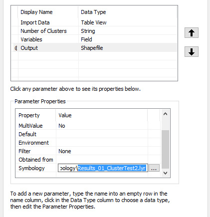
The next window is very important, because it allows us to set the input and output parameters that will then be passed to R. As we saw in the R script here I set 4 parameters, 3 inputs and 1 output. It is important that the order matches what we have in the R script, so for example the number of clusters is the second input.

The first parameter is the input data. For this I used the type "Table View", which allows the user to select a dataset s/he already imported in ArcGIS. I selected this because usually I first load data into ArcGIS, check them, and then perform some analysis. However, if you prefer I think you could also select the type shapefile, to allow users to select a shp directly from their PC.
The next parameter is the number of clusters, which is a simple number. Then we have the field variables. This is very important because we need to set it in a way that allow users to select variables directly from the dataset we are importing.

We can do that by setting the options "Filter" and "Obtained from" that you see in the image above. It is important that we set "Obtained from" with the name of our input data.
At this point we can set the output file, which is a shapefile.

One thing we could do is set the symbology for the shapefile that will be created at the end of the script. To do so we need to create and set a layer file. I did it by changing the symbology to another shapefile and then export it. The only problem is that this technique is not really flexible, meaning that if the layer is set for 5 clusters and users select 10, the symbology will still be with 5 colors. I am not sure if that can be changed or adapted somehow. If the symbology file is not provided the R script will still run correctly and produce a result, but this will not have any colors and users will need to set these afterwards, which probably is not a big deal.
Once this final step is done we can finish the creation of the tool and take a look at the resulting GUI:

Run the Toolbox
Now that we have created both the script and the Toolbox to run it, we can test it. I included a shapefile with the location of Earthquakes that I downloaded from the USGS website yesterday (01 July 2016). This way you can test the tool with real data. As variables you can select: depth, magnitude, distance from volcanoes, faults and tectonic plates. For more info on this dataset please look at one of my previous posts: http://r-video-tutorial.blogspot.ch/2015/06/cluster-analysis-on-earthquake-data.html
We only need to fill the values in the GUI and then click OK. You can see the result in the image below:

As you can see R first produces a histogram of the variable/s the user selects, which can be saved. Then creates a shapefile that is automatically imported in ArcGIS. Moreover, as you can see from the dialog box, we can use the function print to provide messages to the user. Here I put only some simple text, but it may well be some numerical results.

Source Code
The source code for this Toolbox is provided in my GitHub at this link:
https://github.com/fveronesi/Clustering_Toolbox