Showing posts with label xts. Show all posts

Friday, 15 July 2016

Time Series Analysis in ArcGIS

In this post I will introduce another toolbox I created to show the functions that can be added to ArcGIS by using R and the R-Bridge technology.
In this toolbox I basically implemented the functions I showed in the previous post about time series analysis in R.
Once again I prepared a sample dataset that I included in the GitHub archive so that you can reproduce the experiment I'm presenting here. I will start my description from there.

Dataset
As for my previous post, here I'm also including open data in shapefile from the EPA, which I downloaded for free using the custom R function I presented here.
I downloaded only temperature data (in F) from 2013, but I kept two categorical variables: State and Address.


As you can see from the image above the time variable is in the format year-month-day. As I mentioned in the post about the plotting toolbox, it is important to set this format correctly so that R can recognize it. Please refer to this page for more information about the formats that R recognizes.


Time Series Plot
This type of plot is available in several packages, including ggplot2, which I used to create the plotting toolbox.  However, in my post about time series analysis I presented the package xts, which is very powerful for handling and plotting time-series data. For this toolbox I decided to maintain the same package and refer everything to xts for several reasons that I would explain along the text.
The first reason is related to the plotting capabilities of this package. Let's take a look for example at the first script in the toolbox, specific for plotting time series.


Similarly to the script for time series in the plotting toolbox, here users need to select the dataset (which can be a shapefile or a CSV, or any other table format that can be accessed in ArcGIS). Then they need to select the variable of interest, in the sample dataset that is Temp, which clearly stands for temperature. Another important information for R is the data/time column and its format, again please refer to my previous post for more information. Finally, I inserted an SQL call to subset the dataset. In this case I'm subsetting a particular station.
The result is the plot below:


As you can see there are quite a few missing values in the dataset related to the station I subset. The very nice thing about the package xts is that with this plot it is perfectly clear where are the missing data, since along the X axis these are evident by the lack of grey tick marks.


Time Histogram
This is a simple bar chart that basically plots time against frequency of samples. The idea behind this plot is to allow users to explore the number of samples for specific time intervals in the dataset.


The user interface is similar to the previous scrips. Users need to select the dataset, then the variable and then the time column and specify its format. I also included an option to select a subset of the dataset with a SQL selection. At this point I included a list to select the averaging period, and users can select between day, month or year. In this case I selected month, which means that R will loop through the months and subset the dataset for each of these. Then it will basically count the number of data sampled in each month and plot this information against the month itself. The result is the plot below:


As you can see we can definitely gather some useful information from this plot; for example we can determine that basically this station, in the year 2013, did not have any problem.


Time Subset
In some cases we may need to subset our dataset according to a particular time period. This can be done in ArcGIS with the "Select by Attribute" tool and by using an SQL string similar to what you see in the image below:


The package xts however, provides much more powerful and probably faster ways to subset by time. For example, in ArcGIS if we want to subset the whole month of June we would need to specify an SQL string like this:
"Time" >= '2013-06-01' AND "Time" < '2013-07-01'

On the contrary, in R and with the package xts if we wanted to do the same we would just need to use the string '2013-06', and R would know to keep only the month of June. Below are some other examples of successful time subset with the package xts (from http://www.inside-r.org/packages/cran/xts/docs/xts):

sample.xts['2013']  # all of 2013
sample.xts['2013-03']  # just March 2013
sample.xts['2013-03/']  # March 2013 to the end of the data set
sample.xts['2013-03/2013']  # March 2013 to the end of 2013
sample.xts['/'] # the whole data set
sample.xts['/2013'] # the beginning of the data through 2013
sample.xts['2013-01-03'] # just the 3rd of January 2013


With this in mind I created the following script:


As you can see from the image above, here there is an option named "Subset" where users can insert one of the strings from the examples above (just the text within square brackets) and select time intervals with the same flexibility allowed in R and the package xts.
The result of this script is a new shapefile containing only the time included in the Subset call.


Time Average Plots
As I showed in my previous post about time series analysis, with the package xts is possible to perform custom functions on specific time intervals with the following commands: apply.daily, apply.weekly, apply.monthly and apply.yearly.
In this toolbox I used these functions to compute the average, 25th and 75th percentiles for specific time intervals, which the user may choose. This is the toolbox:


The only differences from the other scripts are the "Average by", with which the user can select between day, week, month or year. Each of these will trigger the appropriate apply function. Then there is also the possibility to select the position for the plot legend: between topright, topleft, bottomright and bottomleft. Finally, users can select the output folder where the plot below will be saved, along with a CSV with the numerical values for mean, q25 and q75.


Time Function
This is another script that provides direct access to the apply functions I presented before. Here the output is not a plot but a CSV with the results of the function, and users can input their own function directly in the GUI. Let's take a look:


As you can see there is a field named "Function". Here users can insert their own custom function, written in the R language. This function takes a vector (x) and returns a vector and it is in the form:

function(x){sum(x>70}

Only the string within curly brackets needs to be written in the GUI. This will then be passed to the script and applied to the values averaged by day, week, month or year. Users can select this last aspect in the field "Average by". Here for example I am calculating the number of days, for each month, with a temperature above 70 degrees Fahrenheit (21 degrees celsius) in Alaska. The results are saved in CSV in the output folder and printed on screen, as you can see from the image below.


Trend Analysis
In this last script I included access to the function decompose, which I briefly described in my previous post. This function does not work with xts time series, so the time series needs to be loaded with the standard method, ts, in R. This method requires the user to include the frequency of the time series. For this reason I had to add an option for this in the GUI.
Unfortunately, the dataset I created for this experiment only has one full year and thus making a decomposition does not make much sense, but you are invited to try with your data and it should work fine and provide you with results similar to the image below:


Download
Once again the time-series toolbox is available for free from my GitHub page at:
https://github.com/fveronesi/TimeSeries_Toolbox/

Monday, 18 May 2015

Introductory Time-Series analysis of US Environmental Protection Agency (EPA) pollution data

Download EPA air pollution data
The US Environmental Protection Agency (EPA) provides tons of free data about air pollution and other weather measurements through their website. An overview of their offer is available here: http://www.epa.gov/airdata/

The data are provided in hourly, daily and annual averages for the following parameters:
Ozone, SO2, CO,NO2, Pm 2.5 FRM/FEM Mass, Pm2.5 non FRM/FEM Mass, PM10, Wind, Temperature, Barometric Pressure, RH and Dewpoint, HAPs (Hazardous Air Pollutants), VOCs (Volatile Organic Compounds) and Lead.

All the files are accessible from this page:
http://aqsdr1.epa.gov/aqsweb/aqstmp/airdata/download_files.html

The web links to download the zip files are very similar to each other, they have an initial starting URL: http://aqsdr1.epa.gov/aqsweb/aqstmp/airdata/
and then the name of the file has the following format: type_property_year.zip
The type can be: hourly, daily or annual. The properties are sometimes written as text and sometimes using a numeric ID. Everything is separated by an underscore.

Since these files are identified by consistent URLs I created a function in R that takes year, property and type as arguments, downloads and unzip the data (in the working directory) and read the csv.
To complete this experiment we would need the following packages: sp, raster, xts, plotGoogleMaps
The code for this function is the following:

download.EPA <- function(year, property = c("ozone","so2","co","no2","pm25.frm","pm25","pm10","wind","temp","pressure","dewpoint","hap","voc","lead"), type=c("hourly","daily","annual")){
if(property=="ozone"){PROP="44201"}
if(property=="so2"){PROP="42401"}
if(property=="co"){PROP="42101"}
if(property=="no2"){PROP="42602"}
 
if(property=="pm25.frm"){PROP="88101"}
if(property=="pm25"){PROP="88502"}
if(property=="pm10"){PROP="81102"}
 
if(property=="wind"){PROP="WIND"}
if(property=="temp"){PROP="TEMP"}
if(property=="pressure"){PROP="PRESS"}
if(property=="dewpoint"){PROP="RH_DP"}
if(property=="hap"){PROP="HAPS"}
if(property=="voc"){PROP="VOCS"}
if(property=="lead"){PROP="lead"}
 
URL <- paste0("https://aqs.epa.gov/aqsweb/airdata/",type,"_",PROP,"_",year,".zip")
download.file(URL,destfile=paste0(type,"_",PROP,"_",year,".zip"))
unzip(paste0(type,"_",PROP,"_",year,".zip"),exdir=paste0(getwd()))
read.table(paste0(type,"_",PROP,"_",year,".csv"),sep=",",header=T)
}

This function can be used as follow to create a data.frame with exactly the data we are looking for:

data <- download.EPA(year=2013,property="ozone",type="daily")

This creates a data.frame object with the following characteristics:

> str(data)
'data.frame':   390491 obs. of  28 variables:
 $ State.Code         : int  1 1 1 1 1 1 1 1 1 1 ...
 $ County.Code        : int  3 3 3 3 3 3 3 3 3 3 ...
 $ Site.Num           : int  10 10 10 10 10 10 10 10 10 10 ...
 $ Parameter.Code     : int  44201 44201 44201 44201 44201 44201 44201 44201 44201 44201 ...
 $ POC                : int  1 1 1 1 1 1 1 1 1 1 ...
 $ Latitude           : num  30.5 30.5 30.5 30.5 30.5 ...
 $ Longitude          : num  -87.9 -87.9 -87.9 -87.9 -87.9 ...
 $ Datum              : Factor w/ 4 levels "NAD27","NAD83",..: 2 2 2 2 2 2 2 2 2 2 ...
 $ Parameter.Name     : Factor w/ 1 level "Ozone": 1 1 1 1 1 1 1 1 1 1 ...
 $ Sample.Duration    : Factor w/ 1 level "8-HR RUN AVG BEGIN HOUR": 1 1 1 1 1 1 1 1 1 1 ...
 $ Pollutant.Standard : Factor w/ 1 level "Ozone 8-Hour 2008": 1 1 1 1 1 1 1 1 1 1 ...
 $ Date.Local         : Factor w/ 365 levels "2013-01-01","2013-01-02",..: 59 60 61 62 63 64 65 66 67 68 ...
 $ Units.of.Measure   : Factor w/ 1 level "Parts per million": 1 1 1 1 1 1 1 1 1 1 ...
 $ Event.Type         : Factor w/ 3 levels "Excluded","Included",..: 3 3 3 3 3 3 3 3 3 3 ...
 $ Observation.Count  : int  1 24 24 24 24 24 24 24 24 24 ...
 $ Observation.Percent: num  4 100 100 100 100 100 100 100 100 100 ...
 $ Arithmetic.Mean    : num  0.03 0.0364 0.0344 0.0288 0.0345 ...
 $ X1st.Max.Value     : num  0.03 0.044 0.036 0.042 0.045 0.045 0.045 0.048 0.057 0.059 ...
 $ X1st.Max.Hour      : int  23 10 18 10 9 10 11 12 12 10 ...
 $ AQI                : int  25 37 31 36 38 38 38 41 48 50 ...
 $ Method.Name        : Factor w/ 1 level " - ": 1 1 1 1 1 1 1 1 1 1 ...
 $ Local.Site.Name    : Factor w/ 1182 levels ""," 201 CLINTON ROAD, JACKSON",..: 353 353 353 353 353 353 353 353 353 353 ...
 $ Address            : Factor w/ 1313 levels "  Edgewood  Chemical Biological Center (APG), Waehli Road",..: 907 907 907 907 907 907 907 907 907 907 ...
 $ State.Name         : Factor w/ 53 levels "Alabama","Alaska",..: 1 1 1 1 1 1 1 1 1 1 ...
 $ County.Name        : Factor w/ 631 levels "Abbeville","Ada",..: 32 32 32 32 32 32 32 32 32 32 ...
 $ City.Name          : Factor w/ 735 levels "Adams","Air Force Academy",..: 221 221 221 221 221 221 221 221 221 221 ...
 $ CBSA.Name          : Factor w/ 414 levels "","Adrian, MI",..: 94 94 94 94 94 94 94 94 94 94 ...
 $ Date.of.Last.Change: Factor w/ 169 levels "2013-05-17","2013-07-01",..: 125 125 125 125 125 125 125 125 125 125 ...

The csv file contains a long series of columns that should again be consistent among all the dataset cited above, even though it changes slightly between hourly, daily and annual average.
A complete list of the meaning of all the columns is available here:
aqsdr1.epa.gov/aqsweb/aqstmp/airdata/FileFormats.html

Some of the columns are self explanatory, such as the various geographical names associated with the location of the measuring stations. For this analysis we are particularly interested in the address (that we can use to extract data from individual stations), event type (that tells us if extreme weather events are part of the averages), the date and the actual data (available in the column Arithmetic.Mean).


Extracting data for individual stations
The data.frame we loaded using the function download.EPA contains Ozone measurements from all over the country. To perform any kind of analysis we first need a way to identify and then subset the stations we are interested in.
For doing so I though about using one of the interactive visualization I presented in the previous post. To use that we first need to transform the csv into a spatial object. We can use the following loop to achieve that:

locations <- data.frame(ID=numeric(),LON=numeric(),LAT=numeric(),OZONE=numeric(),AQI=numeric())
for(i in unique(data$Address)){
dat <- data[data$Address==i,]
locations[which(i==unique(data$Address)),] <- data.frame(which(i==unique(data$Address)),unique(dat$Longitude),unique(dat$Latitude),round(mean(dat$Arithmetic.Mean,na.rm=T),2),round(mean(dat$AQI,na.rm=T),0))
}
 
locations$ADDRESS <- unique(data$Address)
 
coordinates(locations)=~LON+LAT
projection(locations)=CRS("+init=epsg:4326")

First of all we create an empty data.frame declaring the type of variable for each column. With this loop we can eliminate all the information we do not need from the dataset and keep the one we want to show and analyse. In this case I kept Ozone and the Air Quality Index (AQI), but you can clearly include more if you wish.
In the loop we iterate through the addresses of each EPA station, for each we first subset the main dataset to keep only the data related to that station and then we fill the data.frame with the coordinates of the station and the mean values of Ozone and AQI.
When the loop is over (it may take a while!), we can add the addresses to it and transform it into a SpatialObject. We also need to declare the projection of the coordinates, which in WGS84.
Now we are ready to create an interactive map using the package plotGoogleMaps and the Google Maps API. We can simply use the following line:

map <- plotGoogleMaps(locations,zcol="AQI",filename="EPA_GoogleMaps.html",layerName="EPA Stations")

This creates a map with a marker for each EPA station, coloured with the mean AQI. If we click on a marker we can see the ID of the station, the mean Ozone value and the address (below). The EPA map I created is shown at this link: EPA_GoogleMaps


From this map we can obtain information regarding the EPA stations, which we can use to extract values for individual stations from the dataset.
For example, we can extract values using the ID we created in the loop or the address of the station, which is also available on the Google Map, using the code below:

ID = 135
Ozone <- data[paste(data$Address)==unique(data$Address)[ID]&paste(data$Event.Type)=="None",]
 
ADDRESS = "966 W 32ND"
Ozone <- data[paste(data$Address)==ADDRESS&paste(data$Event.Type)=="None",] 

Once we have extracted only data for a single station we can proceed with the time-series analysis.


Time-Series Analysis
There are two ways to tell R that a particular vector or data.frame is in fact a time-series. We have the function ts available in the package basic and the function xts, available in the package xts.
I will first analyse how to use xts, since this is probably the best way of handling time-series.
The first thing we need to do is make sure that our data have a column of class Date. This is done by transforming the current date values into the proper class. The EPA datasets has a Date.local column that R reads as factors:

> str(Ozone$Date.Local)
 Factor w/ 365 levels "2013-01-01","2013-01-02",..: 90 91 92 93 94 95 96 97 98 99 ...

We can transform this into the class Date using the following line, which creates a new column named DATE in the Ozone object:

Ozone$DATE <- as.Date(Ozone$Date.Local)

Now we can use the function xts to create a time-series object:

Ozone.TS <- xts(x=Ozone$Arithmetic.Mean,order.by=Ozone$DATE)
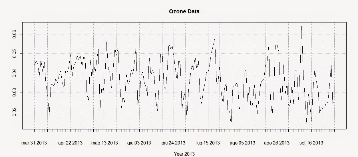
plot(Ozone.TS,main="Ozone Data",sub="Year 2013")

The first line creates the time-series using the Ozone data and the DATE column we created above. The second line plots the time-series and produces the image below:


To extract the dates of the object Ozone we can use the function index and we can use the function coredata to extract the ozone values.

index(Ozone.TS)
 Date[1:183], format: "2013-03-31" "2013-04-01" "2013-04-02" "2013-04-03" ...
 
coredata(Ozone.TS)
 num [1:183, 1] 0.044 0.0462 0.0446 0.0383 0.0469 ...


Subsetting the time-series is super easy in the package xts, as you can see from the code below:

Ozone.TS['2013-05-06'] #Selection of a single day
 
Ozone.TS['2013-03'] #Selection of March data
 
Ozone.TS['2013-05/2013-07'] #Selection by time range

The first line extracts values for a single day (remember that the format is year-month-day); the second extracts values from the month of March. We can use the same method to extract values from one particular year, if we have time-series with multiple years.
The last line extracts values in a particular time range, notice the use of the forward slash to divide the start and end of the range.

We can also extract values by attributes, using the functions index and coredata. For example, if we need to know which days the ozone level was above 0.03 ppm we can simply use the following line:

index(Ozone.TS[coredata(Ozone.TS)>0.03,])

The package xts features some handy function to apply custom functions to specific time intervals along the time-series. These functions are: apply.weekly, apply.monthly, apply.quarterly and apply.yearly

The use of these functions is similar to the use of the apply function. Let us look at the example below to clarify:

apply.weekly(Ozone.TS,FUN=mean)
apply.monthly(Ozone.TS,FUN=max)

The first line calculates the mean value of ozone for each week, while the second computes the maximum value for each month. As for the function apply we are not constrained to apply functions that are available in R, but we can define our own:

apply.monthly(Ozone.TS,FUN=function(x) {sd(x)/sqrt(length(x))})

in this case for example we can define a function to calculate the standard error of the mean for each month.

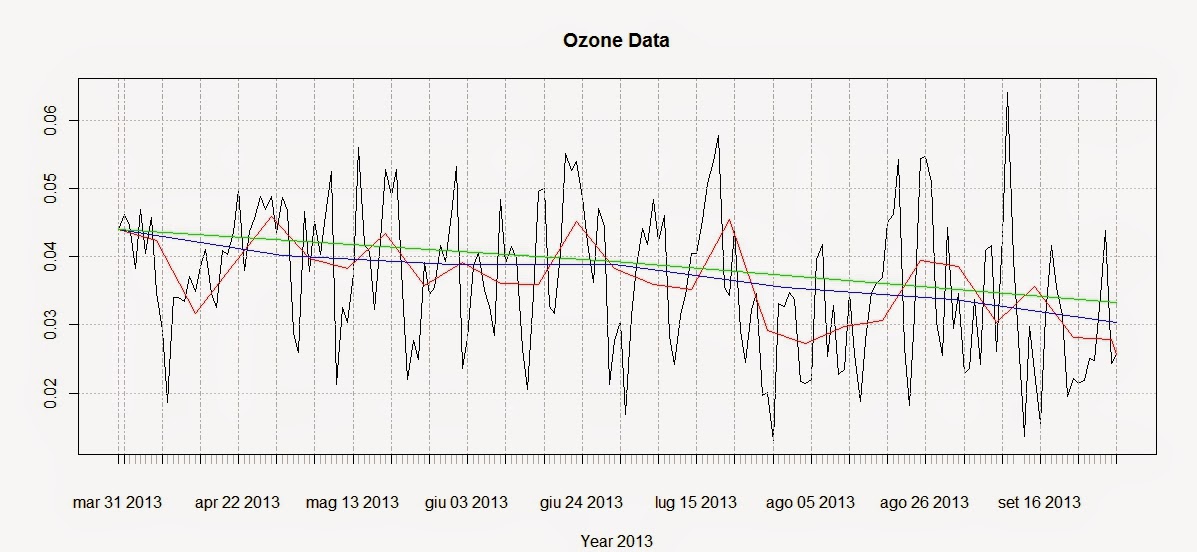
We can use these functions to create a simple plot that shows averages for defined time intervals with the following code:

plot(Ozone.TS,main="Ozone Data",sub="Year 2013")
lines(apply.weekly(Ozone.TS,FUN=mean),col="red")
lines(apply.monthly(Ozone.TS,FUN=mean),col="blue")
lines(apply.quarterly(Ozone.TS,FUN=mean),col="green")
lines(apply.yearly(Ozone.TS,FUN=mean),col="pink")

These lines return the following plot:


From this image it is clear that ozone presents a general decreasing trend over 2013 for this particular station. However, in R there are more precise ways of assessing the trend and seasonality of time-series.

Trends
Let us create another example where we use again the function download.EPA to download NO2 data over 3 years and then assess their trends.

NO2.2013.DATA <- download.EPA(year=2013,property="no2",type="daily")
NO2.2012.DATA <- download.EPA(year=2012,property="no2",type="daily")
NO2.2011.DATA <- download.EPA(year=2011,property="no2",type="daily")
 
ADDRESS = "2 miles south of Ouray and south of the White and Green River confluence"  #Copied and pasted from the interactive map
NO2.2013 <- NO2.2013.DATA[paste(NO2.2013.DATA$Address)==ADDRESS&paste(NO2.2013.DATA$Event.Type)=="None",]
NO2.2012 <- NO2.2012.DATA[paste(NO2.2012.DATA$Address)==ADDRESS&paste(NO2.2012.DATA$Event.Type)=="None",]
NO2.2011 <- NO2.2011.DATA[paste(NO2.2011.DATA$Address)==ADDRESS&paste(NO2.2011.DATA$Event.Type)=="None",]
 
 
NO2.TS <- ts(c(NO2.2011$Arithmetic.Mean,NO2.2012$Arithmetic.Mean,NO2.2013$Arithmetic.Mean),frequency=365,start=c(2011,1))

The first lines should be clear from we said before. The only change is that the time-series is created using the function ts, available in base R. With ts we do not have to create a column of class Date in our dataset, but we can just specify the starting point of the time series (using the option start, which in this case is January 2011) and the number of samples per year with the option frequency. In this case the data were collected daily so the number of times per year is 365; if we had a time-series with data collected monthly we would specify a frequency of 12.

We can decompose the time-series using the function decompose, which is based on moving averages:

dec <- decompose(NO2.TS)
plot(dec)

The related plot is presented below:


There is also another method, based on the loess smoother (for more info: Article) that can be accessed using the function stl:

STL <- stl(NO2.TS,"periodic")
plot(STL)

This function is able to calculate the trend along the whole length of the time-series:


Conclusions
This example shows how to download and access the open pollution data for the US available from the EPA directly from R.
Moreover we have seen here how to map the locations of the stations and subset the dataset. We also looked at ways to perform some introductory time-series analysis on pollution data.
For more information and material regarding time-series analysis please refer to the following references:

A Little Book of R For Time Series

Analysis of integrated and cointegrated time series with R

Introductory time series with R


R code snippets created by Pretty R at inside-R.org